Processing and Visualizing Data
- In the modern data-driven world, the ability to effectively process and visualize data is crucial. Data processing involves transforming raw data into a meaningful format that can be analyzed and interpreted. Visualization, on the other hand, helps to present this processed data in a graphical format, making it easier to identify patterns, trends, and insights. Together, these skills enable data scientists and analysts to make informed decisions and communicate their findings clearly.
- Two powerful tools that aid in this process are NumPy and pandas. NumPy provides support for large, multi-dimensional arrays and matrices, along with a collection of mathematical functions to operate on these arrays. It forms the foundation for numerical computing in Python. pandas builds on NumPy by offering data structures and operations specifically designed for data manipulation and analysis, making it easier to handle and analyze large datasets. Before diving into the technical aspects like using NumPy for array manipulations, it's important to grasp the fundamental concepts of data processing and visualization, as these form the backbone of data analysis.
NumPy
- NumPy is an open-source library designed for working with arrays.
- The name stands for Numerical Python and it is a critical data science library in Python, with many other libraries depending on it.
- NumPy is extremely popular because it improves the performance of working with multi-dimensional arrays. Mathematical operations on NumPy arrays are up to 50 times faster than iterating over Python lists using loops. It requires fewer lines of code for mathematical operations compared to native Python lists.
- It offers an indexing system for easily accessing portions of data within arrays.
- It contains built-in functions that improve the quality of code when working with arrays and mathematics, such as linear algebra, array transformations, and other mathematical operations.
Purpose of NumPy
- It is mostly used in data analytics for working with arrays and matrices, including multi-dimensional arrays.
- It helps to solve complex mathematical and statistical operations, offering multiple functions for working with 2D matrices and 3D tensors.
NumPy Arrays
- NumPy arrays are used to create n-dimensional arrays, allowing us to solve complex problems in mathematics, statistics, linear algebra, and matrix operations.
- NumPy provides efficient data structures for handling large datasets and performing fast numerical computations.
- With NumPy arrays, we can perform vectorized operations, which are much faster than traditional loop-based operations on Python lists.
- NumPy is widely used in scientific computing, machine learning, data analysis, and other fields due to its speed and convenience.
- It is a package, so first, we have to import it using:
import numpy as np.
Make sure it is installed on your system by using the command:pip install numpy
Working with Arrays
import numpy as np

# Creating a 1D array
a = np.array([1, 2, 3, 4])
print(a)
The above code creates a 1D array and prints it.
Taking elements from the user and printing them:
import numpy as np

# Taking input from the user
n = int(input("Enter the number of elements in the array: "))
elements = []

for i in range(n):
    element = int(input(f"Enter element {i + 1}: "))
    elements.append(element)

# Converting the list of elements to a NumPy array
elements_array = np.array(elements)

print("The created array is:", elements_array)
The above code takes the number of elements and each element from the user to create an array and then prints the array. It prompts the user to enter the number of elements in the array, then iteratively takes each element as input, appends it to a list, converts the list to a NumPy array, and prints the resulting array.
Creating 1D, 2D, and 3D Arrays in NumPy
1. Creating a 1D array:
import numpy as np

# Creating a 1D array using np.array()
a_1d = np.array([1, 2, 3, 4, 5])
print("1D Array:")
print(a_1d)
2. Creating a 2D array:
# Creating a 2D array using np.array()
a_2d = np.array([[1, 2, 3], [4, 5, 6]])
print("2D Array:")
print(a_2d)
3. Creating an 3D array:
# Creating an N-dimensional array using np.array()
a_nd = np.array([[[1, 2], [3, 4]], [[5, 6], [7, 8]]])
print("3D Array:")
print(a_nd)
The above code demonstrates creating 1D, 2D, and 3D arrays in NumPy using the np.array() function. You can specify the elements of the array as nested lists, with each list representing a row in a 2D array or a higher-dimensional structure in N-dimensional arrays.
Special Arrays in NumPy
- NumPy provides functions to easily create special arrays, such as:
1- Zero Array
import numpy as np

# Creating a 1D zero array of length 3
print(np.zeros(3))

# Creating a 2D zero array of shape (3, 3)
print(np.zeros((3, 3)))
Output:
[0. 0. 0.]

[[0. 0. 0.]
[0. 0. 0.]
[0. 0. 0.]]
The np.zeros() function creates an array filled with zeros. When used with a single argument, it creates a 1D array of zeros with the specified length. When used with a tuple specifying the shape, it creates a multi-dimensional array (in this case, a 2D array) filled with zeros.
2. Ones Array: An array where all elements are ones.
import numpy as np

# Creating a 1D ones array of length 3
print(np.ones(3))

# Creating a 2D ones array of shape (3, 3)
print(np.ones((3, 3)))
Output:
[1. 1. 1.]

[[1. 1. 1.]
[1. 1. 1.]
[1. 1. 1.]]
3. Full Array: An array filled with a specified value.
# Creating a 1D full array of length 3 filled with 5
print(np.full(3, 5))

# Creating a 2D full array of shape (3, 3) filled with 7
print(np.full((3, 3), 7))
Output:
[5 5 5]

[[7 7 7]
[7 7 7]
[7 7 7]]
4. Identity Matrix: A square matrix with ones on the diagonal and zeros elsewhere.
# Creating a 3x3 identity matrix
print(np.eye(3))
Output:
[[1. 0. 0.]
[0. 1. 0.]
[0. 0. 1.]]
5. Range Array: An array of evenly spaced values within a specified range.
# Creating a range array from 0 to 5 (exclusive) with a step of 1
print(np.arange(0, 5, 1))

# Creating a range array from 0 to 10 (exclusive) with a step of 2
print(np.arange(0, 10, 2))
Output:
[0 1 2 3 4]

[0 2 4 6 8]
Attributes of NumPy Arrays
1. ndim: The ndim attribute returns the number of dimensions (axes) of the array.
import numpy as np

# Creating a NumPy array
a = np.array([[1, 2, 3], [4, 5, 6]])

# Using ndim attribute to get the number of dimensions
num_dimensions = a.ndim
print("Number of dimensions:", num_dimensions)
The ndim attribute in this example will return 2, indicating that the array 'a' is a 2-dimensional array.
2. shape: The shape attribute returns a tuple representing the shape of the array.
# Using shape attribute to get the shape of the array
array_shape = a.shape
print("Shape of the array:", array_shape)
The shape attribute will return (2, 3), indicating that the array 'a' has 2 rows and 3 columns.
3. size: The size attribute returns the total number of elements in the array.
# Using size attribute to get the total number of elements
array_size = a.size
print("Size of the array:", array_size)
The size attribute will return 6, indicating that the array 'a' contains 6 elements.
4. dtype: The dtype attribute returns the data type of the elements in the array.
# Using dtype attribute to get the data type of elements
array_dtype = a.dtype
print("Data type of the array:", array_dtype)
The dtype attribute will return int64, indicating that the elements in the array 'a' are of type integer with 64-bit precision.
These attributes provide valuable information about the structure, size, and data type of NumPy arrays, allowing for effective manipulation and analysis of array data.
Upcasting in NumPy
When performing operations or combining arrays with different data types in NumPy, there is a concept called "upcasting" where NumPy automatically converts the data types of the arrays to a common data type to ensure consistency.
Example:
import numpy as np

# Creating arrays with different data types
a = np.array([1, 2, 3])
b = np.array([1.1, 2.2, 3.3])

# Performing an operation that requires upcasting
c = a + b

print("Array a (int):", a)
print("Array b (float):", b)
print("Array c (upcasted):", c)
print("Data type of array c:", c.dtype)
In this example, array 'a' has integer elements, and array 'b' has floating-point elements. When we perform the addition operation (a + b), NumPy automatically upcasts the elements of array 'a' to float64 to match the data type of array 'b', resulting in array 'c' with elements of type float64.
The output will show the arrays and their data types, confirming the upcasting that occurred during the operation.
Understanding upcasting is important when working with mixed data types in NumPy arrays to ensure correct results and avoid unexpected behavior due to data type inconsistencies.
Handling Mixed Data Types in NumPy Arrays
NumPy arrays can handle mixed data types, but it's essential to understand how NumPy treats these mixed types, especially during operations and array creation.
Example 1: Integer and Float Elements
import numpy as np

# Creating an array with integer and float elements
mixed_array = np.array([2, 3, 4.4, 4, 3])

print("Mixed-type array:", mixed_array)
print("Data type of the array:", mixed_array.dtype)
Output:
Mixed-type array: [2.  3.  4.4 4.  3. ]
Data type of the array: float64
In this example, the array contains both integers and floats. NumPy automatically upcasts the integers to floating-point numbers to maintain consistency in operations, resulting in the entire array being of data type float64.
Example 2: Integer and String Elements
# Creating an array with integer and string elements
mixed_array = np.array([3, 4, 5, '6', 4])

print("Mixed-type array:", mixed_array)
print("Data type of the array:", mixed_array.dtype)
Output:
Mixed-type array: ['3' '4' '5' '6' '4']
Data type of the array: <U21
Here, the array contains integers and a string. NumPy upcasts the entire array to a string data type (<U21) because of the presence of a string element, ensuring consistency in the array's data type.
Understanding how NumPy handles mixed data types is crucial for avoiding unexpected behavior and ensuring correct data processing in array operations and manipulations.
Creating N-dimensional Arrays with ndmin
- The ndmin argument in np.array specifies the minimum number of dimensions an array should have.
import numpy as np

# Create a 1D array
arr = np.array([1, 2, 3])

# Increase the dimension of the array to 5 using ndmin argument
ndimarray = np.array(arr, ndmin=5)

# Print the shape of the new array
print(ndimarray.shape)
- np.array(arr, ndmin=5) creates a new array from arr and ensures it has a minimum of 5 dimensions using ndmin=5
- By specifying ndmin=5, NumPy adds four additional dimensions at the beginning, each of size 1.
- the resulting array has a shape of (1, 1, 1, 1, 3). Each 1 corresponds to a new dimension added by the ndmin parameter, and the final dimension 3 corresponds to the original array's length.
Random Number Generation in Numpy
- NumPy provides a suite of functions for generating random numbers and performing random operations. These functions are part of the numpy.random module.
- Role of Random Number Generation in NumPy:
- Simulations and Modeling : Random numbers are essential for creating simulations that mimic real-world phenomena, such as weather patterns, financial markets, or physical processes. For example, Monte Carlo simulations rely heavily on random number generation to model complex systems and assess the impact of uncertainty.
- Statistical Analysis : Random numbers are used in statistical methods such as bootstrapping and resampling to estimate the distribution of a statistic by sampling with replacement from the original data.
- Machine Learning: In machine learning, random numbers are used for initializing weights in neural networks, splitting datasets into training and testing sets, shuffling data, and augmenting data to improve model robustness.
- Random Sampling: Random number generation allows for the creation of random samples from larger datasets, which is useful for exploratory data analysis, hypothesis testing, and creating training datasets.
- Data Augmentation: In fields like computer vision and natural language processing, random transformations such as rotations, translations, or noise addition are applied to data to create new training samples, enhancing model generalization.
- Cryptography: Although cryptographically secure random numbers should be generated using specialized libraries, random number generation in NumPy can be used for simulations and prototyping cryptographic algorithms.
- Games and Entertainment : Random numbers are used to introduce unpredictability and variation in games, such as shuffling cards, rolling dice, or generating random game scenarios.
- Algorithm Testing: Random number generation is used to create test cases and benchmark algorithms, ensuring they perform well under different conditions and inputs.
Basic Random Number Generation
- Generating Random Floats: The rand() function generates random floats between 0
and 1.
import numpy as np random_floats = np.random.rand(3) # Generates an array of 3 random floats print(random_floats)[0.37454012 0.95071431 0.73199394] - Generating Random Integers: The randint() function generates random integers
within a specified range.
random_integers = np.random.randint(1, 10, size=5) # Generates an array of 5 random integers between 1 and 9 print(random_integers)[8 1 5 9 3]
Creating Random Arrays
- Random Array of Given Shape: The rand() function can also be used to create
random arrays of a given shape.
random_array = np.random.rand(2, 3) # Generates a 2x3 array of random floats print(random_array)[[0.59865848 0.15601864 0.15599452] [0.05808361 0.86617615 0.60111501]] - Random Integer Array of Given Shape: The randint() function can be used to
create arrays of random integers.
random_int_array = np.random.randint(1, 100, size=(2, 3)) # Generates a 2x3 array of random integers between 1 and 99 print(random_int_array)[[12 84 56] [78 60 38]]
Array Indexing and Slicing
1D Array Indexing (Single Dimension)
Basic rules:
- Indexing starts at 0 (first element is index 0)
- Negative indices count from the end (-1 is the last element)
- Slicing uses [start:stop:step] format
import numpy as np

# Create a simple 1D array
numbers = np.array([10, 20, 30, 40, 50, 60, 70, 80, 90])
print("Original array:", numbers)

# Getting single elements
print("First element (index 0):", numbers[0])      # 10
print("Third element (index 2):", numbers[2])      # 30
print("Last element (index -1):", numbers[-1])     # 90
print("Second to last (index -2):", numbers[-2])   # 80

# Getting multiple elements (slicing)
print("First 3 elements:", numbers[:3])        # [10, 20, 30]
print("Last 3 elements:", numbers[-3:])        # [70, 80, 90]
print("Elements 2 to 5:", numbers[2:6])        # [30, 40, 50, 60]
print("Every 2nd element:", numbers[::2])      # [10, 30, 50, 70, 90]
print("Every 3rd element:", numbers[::3])      # [10, 40, 70]
print("Reverse order:", numbers[::-1])         # [90, 80, 70, 60, 50, 40, 30, 20, 10]

# Changing values
numbers[0] = 100  # Change first element
print("After changing first element:", numbers)

# Change multiple values at once
numbers[1:4] = [200, 300, 400]
print("After changing elements 1-3:", numbers)
Now we do in 2d Array
- So, let's create a 2D array:
import numpy as np

# Create a 1D array with values from 1 to 50
a = np.arange(1, 51)

# Reshape the 1D array to a 2D array with 10 rows and 5 columns
a = a.reshape(10, 5)
-
a = np.arange(1, 51)will create a 1D array that starts from 1 and goes up to 50 as follows:[1, 2, 3, ..., 50] -
a.reshape(10, 5)will reshape the 1D array into a 2D array with 10 rows and 5 columns as follows:[[ 1, 2, 3, 4, 5], [ 6, 7, 8, 9, 10], [11, 12, 13, 14, 15], [16, 17, 18, 19, 20], [21, 22, 23, 24, 25], [26, 27, 28, 29, 30], [31, 32, 33, 34, 35], [36, 37, 38, 39, 40], [41, 42, 43, 44, 45], [46, 47, 48, 49, 50]]
Now, let's perform some indexing and slicing operations on the 2D array:
- Printing the first array, as this is now an array of arrays, and we are interested in printing
the first row:
print(a[0])[ 1, 2, 3, 4, 5] - Printing the 3rd row array, which will be indexed as 2:
print(a[2])[11, 12, 13, 14, 15] - a[0, 0] - What will this print? 0, 0 means the 0th row
(first row for our
understanding) and 0th column (1st column):
print(a[0, 0])1 - What will a[3, 4] print? It will print the element at the
3rd row and 4th column:
print(a[3, 4])20 - a[2:5] - What does this : represent? That means slicing from
the 2nd
index (inclusive) to the 5th index (exclusive), which will give us rows 3 to 4:
print(a[2:5])[[11, 12, 13, 14, 15], [16, 17, 18, 19, 20], [21, 22, 23, 24, 25]] - Printing all the rows:
print(a[0:10])[[ 1, 2, 3, 4, 5], [ 6, 7, 8, 9, 10], [11, 12, 13, 14, 15], [16, 17, 18, 19, 20], [21, 22, 23, 24, 25], [26, 27, 28, 29, 30], [31, 32, 33, 34, 35], [36, 37, 38, 39, 40], [41, 42, 43, 44, 45], [46, 47, 48, 49, 50]] - Printing a column: a[:, 2] - The first part before , is
for rows,
and after it is for columns. : means all rows, and 2 means
the 3rd column:
print(a[:, 2])[ 3, 8, 13, 18, 23, 28, 33, 38, 43, 48] - a[2:5, 4] - This means selecting rows from index 2 to 4 and the element in
the
4th column:
print(a[2:5, 4])[15, 20, 25] - a[:, :] - This means selecting all rows and all columns:
print(a[:, :])[[ 1, 2, 3, 4, 5], [ 6, 7, 8, 9, 10], [11, 12, 13, 14, 15], [16, 17, 18, 19, 20], [21, 22, 23, 24, 25], [26, 27, 28, 29, 30], [31, 32, 33, 34, 35], [36, 37, 38, 39, 40], [41, 42, 43, 44, 45], [46, 47, 48, 49, 50]] - a[:, 2:5] - This means selecting all rows and columns from index 2 to 4:
print(a[:, 2:5])[[ 3, 4, 5], [ 8, 9, 10], [13, 14, 15], [18, 19, 20], [23, 24, 25], [28, 29, 30], [33, 34, 35], [38, 39, 40], [43, 44, 45], [48, 49, 50]] - a[:, 2:].dtype - This will give the data type of the elements in the array
starting from column index 2 to the end:
print(a[:, 2:].dtype)dtype('int64')
Data Handling using Pandas 🐼
Pandas: A Library for Data Analysis and Manipulation
Overview
- Pandas: It is a package useful for data analysis and manipulation.
- Pandas provides an easy way to create, manipulate, and wrangle data. Wrangling refers to the process of cleaning, transforming, and enriching raw data into a more usable format for analysis.
- Pandas provides powerful and easy-to-use data structures, as well as the means to quickly perform operations on these structures.
Advantages of Pandas
- Easily handles missing data: Pandas provides robust methods to handle missing data efficiently.
- Data Structures: It uses Series for one-dimensional data structure and DataFrame for multi-dimensional data structure.
- Efficient Data Slicing: It provides an efficient way to slice the data.
- Flexible Data Operations: It provides a flexible way to merge, concatenate, or reshape the data.
Installation
- Pandas must be installed first before you can use it in your system:
pip install pandas
- Once installed, it is now ready to be imported and used:
import pandas as pd
Data Structures in Pandas
A data structure is a way to arrange the data so it can be accessed quickly and we can perform various operations on this data like retrieval, deletion, modification, etc.
Pandas deals with three data structures:
- ★ Series: A one-dimensional data structure.
- ★ DataFrame: A multi-dimensional data structure.
- Panel: A three-dimensional data structure (though it is less commonly used and considered deprecated).
Series
A Series is a one-dimensional array-like structure with homogeneous data, which can be used to handle and manipulate data. What makes it special is its index attribute, which has incredible functionality and is heavily mutable.
It has two parts:
- Data part: An array of actual data.
- Associated index with data: An associated array of indexes or data labels.
For example:
Index   Data
0       10
1       15
2       18
3       22
- Series is a labeled one-dimensional array that can hold any type of data.
- Data of Series is always mutable: It means it can be changed.
- Size of Data of Series is always immutable: It means it cannot be changed.
- Series may be considered as a Data Structure with two arrays: One array works as Index (Labels) and the second array works as original Data.
- Row Labels in Series are called Index.
Pandas Series with Python Lists
- A list in Python is a collection of elements which can include integers, strings, floats, and other data types. Lists are mutable and ordered.
lst = [1, 2, 3, 4, 5, 6]
print(lst)
Output:
[1, 2, 3, 4, 5, 6]
There are some advantages of Series over lists:
- Pandas Series provide more functionality, such as the ability to handle missing data, vectorized operations, and the ability to use labels for indexing.
We can create a Series using a list:
import pandas as pd
series = pd.Series(lst)
print(series)
print(type(series))
Output:
0    1
1    2
2    3
3    4
4    5
5    6
dtype: int64
<class 'pandas.core.series.Series'>
- As you can see in the output, the 1D array is converted to a column with an index.
- We can create a Series using a dictionary as well:
data = {'a': 10, 'b': 20, 'c': 30}
series_dict = pd.Series(data)
print(series_dict)
Output:
a    10
b    20
c    30
dtype: int64
Creating Empty Series
- You don't have to provide anything; just an empty list or array.
- By default, the data type is float.
empty = pd.Series([])
print(empty)
Output:
Series([], dtype: float64)
Defining Your Own Index
a = pd.Series(['p', 'q', 'r', 's', 't'], index=[10, 11, 12, 13, 14])
print(a)
Output:
10    p
11    q
12    r
13    s
14    t
dtype: object
Giving Name to a Series
- Using this we can assign a name to the Series, which can be useful for identifying the Series in a DataFrame or when displaying it.
a = pd.Series(['p', 'q', 'r', 's', 't'], index=[10, 11, 12, 13, 14], name="alphabets")
print(a)
Output:
10    p
11    q
12    r
13    s
14    t
Name: alphabets, dtype: object
Creating Scalar Series
- A scalar Series is a Series where every element is the same scalar value.
scalar_series = pd.Series(0.5)
print(scalar_series)
Output:
0    0.5
dtype: float64
- This contains a single scalar value 0.5 repeated once.
Increasing the Quantity of the Scalar Values
- We can do this by specifying an index with the desired length.
scalar_series = pd.Series(0.5, index=[1, 2, 3])
print(scalar_series)
Output:
1    0.5
2    0.5
3    0.5
dtype: float64
Pandas Series with Python Dictionary
- A dictionary in Python contains key-value pairs, where each key is unique and maps to a corresponding value.
Creating a Series using a dictionary:
import pandas as pd
dict_series = pd.Series({'p': 1, 'q': 2, 'r': 3, 's': 4, 't': 5})
print(dict_series)
Output:
p    1
q    2
r    3
s    4
t    5
dtype: int64
Accessing the Data
print(dict_series[0])
Output:
1
- This will print the value associated with the first key in the Series, which is 1.
print(dict_series[0:3])
Output:
p    1
q    2
r    3
dtype: int64
- This will print the first three elements in the Series.
Getting the Maximum Value in the Series
print(max(dict_series))
Output:
5
Increasing the Column Count
- Till now, it was containing only one column. Now we want three columns, and we can do this by combining a dictionary and a list.
dict_series = pd.Series({'p': [1, 5, 6], 'q': [2, 6, 7], 'r': [3, 7, 8], 's': [4, 8, 9], 't': [5, 9, 10]})
print(dict_series)
Output:
p    [1, 5, 6]
q    [2, 6, 7]
r    [3, 7, 8]
s    [4, 8, 9]
t    [5, 9, 10]
dtype: object
Mathematical Operations in Series
Pandas Series supports various mathematical operations. These operations are performed element-wise and are very similar to numpy array operations. Let's discuss the common mathematical operations using a single program.
Program:
import pandas as pd
import numpy as np

# Creating a Series
series = pd.Series([10, 20, 30, 40, 50])

# Multiplication by a scalar
multiplication = series * 2

# Square of each element
square = series ** 2

# Filtering values greater than 25
greater_than_25 = series[series > 25]

print("Original Series:")
print(series)
print("\nMultiplication by 2:")
print(multiplication)
print("\nSquare of each element:")
print(square)
print("\nValues greater than 25:")
print(greater_than_25)
Output:
Original Series:
0    10
1    20
2    30
3    40
4    50
dtype: int64

Multiplication by 2:
0     20
1     40
2     60
3     80
4    100
dtype: int64

Square of each element:
0     100
1     400
2     900
3    1600
4    2500
dtype: int64

Values greater than 25:
2    30
3    40
4    50
dtype: int64
Mathematical operation involving 2 series
Program:
import pandas as pd
import numpy as np

# Creating two Series
series1 = pd.Series([10, 20, 30, 40, 50])
series2 = pd.Series([5, 10, 15, 20, 25])

# Addition
addition = series1 + series2

# Subtraction
subtraction = series1 - series2

# Multiplication
multiplication = series1 * series2

# Division
division = series1 / series2

# Exponentiation
exponentiation = series1 ** 2

# Modulus
modulus = series1 % 3

print("Series 1:")
print(series1)
print("\nSeries 2:")
print(series2)
print("\nAddition:")
print(addition)
print("\nSubtraction:")
print(subtraction)
print("\nMultiplication:")
print(multiplication)
print("\nDivision:")
print(division)
print("\nExponentiation:")
print(exponentiation)
print("\nModulus:")
print(modulus)
Output:
Series 1:
0    10
1    20
2    30
3    40
4    50
dtype: int64

Series 2:
0     5
1    10
2    15
3    20
4    25
dtype: int64

Addition:
0    15
1    30
2    45
3    60
4    75
dtype: int64

Subtraction:
0     5
1    10
2    15
3    20
4    25
dtype: int64

Multiplication:
0     50
1    200
2    450
3    800
4    1250
dtype: int64

Division:
0    2.0
1    2.0
2    2.0
3    2.0
4    2.0
dtype: float64

Exponentiation:
0     100
1     400
2     900
3    1600
4    2500
dtype: int64

Modulus:
0    1
1    2
2    0
3    1
4    2
dtype: int64
Head and Tail Functions in Series
Pandas Series provides the head() and tail() functions to easily view a subset of the data. These functions are useful for quickly inspecting the beginning and end of a Series.
Program:
import pandas as pd

# Creating a Series
series = pd.Series([10, 20, 30, 40, 50, 60, 70, 80, 90, 100])

# Using the head() function
head_default = series.head()
head_custom = series.head(3)

# Using the tail() function
tail_default = series.tail()
tail_custom = series.tail(3)

print("Original Series:")
print(series)
print("\nFirst 5 elements (head - default):")
print(head_default)
print("\nFirst 3 elements (head - custom):")
print(head_custom)
print("\nLast 5 elements (tail - default):")
print(tail_default)
print("\nLast 3 elements (tail - custom):")
print(tail_custom)
Output:
Original Series:
0     10
1     20
2     30
3     40
4     50
5     60
6     70
7     80
8     90
9    100
dtype: int64

First 5 elements (head - default):
0    10
1    20
2    30
3    40
4    50
dtype: int64

First 3 elements (head - custom):
0    10
1    20
2    30
dtype: int64

Last 5 elements (tail - default):
5     60
6     70
7     80
8     90
9    100
dtype: int64

Last 3 elements (tail - custom):
7     80
8     90
9    100
dtype: int64
This program demonstrates how to use the head() and tail() functions to inspect the beginning and end of a pandas Series.
- series.head(): By default, retrieves the first 5 elements of the Series.
- series.head(3): Retrieves the first 3 elements of the Series.
- series.tail(): By default, retrieves the last 5 elements of the Series.
- series.tail(3): Retrieves the last 3 elements of the Series.
Selection in Series
Pandas Series provides various methods for selecting data, including loc, iloc, and using index or range.
1. loc
The loc function is used to access a group of rows and columns by labels or a boolean array.
- series.loc[label]: Access a single element in the Series using its label.
- series.loc[start_label:end_label]: Access a range of elements from start_label to end_label (inclusive).
- series.loc[condition]: Access elements based on a boolean condition.
Example:
import pandas as pd

data = {'A': 10, 'B': 20, 'C': 30, 'D': 40}
series = pd.Series(data)

print(series.loc['B'])  # Access element with label 'B'
print(series.loc['B':'D'])  # Access elements from 'B' to 'D' (inclusive)
2. iloc
The iloc function is used for integer-location based indexing, i.e., accessing elements by integer position.
- series.iloc[index]: Access an element at a specific integer index.
- series.iloc[start_index:end_index]: Access a range of elements from start_index to end_index (exclusive).
Example:
print(series.iloc[1])  # Access element at index 1
print(series.iloc[1:3])  # Access elements from index 1 to 2 (exclusive)
3. Using Index or Range
You can also select data using square brackets with index or range.
- series[label]: Access an element using its label.
- series[start_label:end_label]: Access a range of elements using labels (inclusive).
- series[index]: Access an element at a specific index.
- series[start_index:end_index]: Access a range of elements using integer indices (exclusive).
series[-index]: Access an element using negative indexing.
Example:
import pandas as pd

# Creating a Series with labels
label_data = {'A': 10, 'B': 20, 'C': 30, 'D': 40}
label_series = pd.Series(label_data)

# Creating a Series with integer indices
index_data = [10, 20, 30, 40]
index_series = pd.Series(index_data)

# Access element with label 'B'
print(label_series['B'])  # Output: 20

# Access range of elements from 'B' to 'D' (inclusive)
print(label_series['B':'D'])  # Output:
# B    20
# C    30
# D    40

# Access element at index 1
print(index_series[1])  # Output: 20

# Access elements from index 1 to 2 (exclusive)
print(index_series[1:3])  # Output:
# 1    20
# 2    30

# Access element using negative indexing
print(index_series[-1])  # Output: 40
Difference Between loc and iloc
- loc: Accesses elements using labels (names) of the data. It is inclusive, meaning it includes the end label in the selection.
- iloc: Accesses elements using integer indices (positions) of the data. It is exclusive, meaning it excludes the end index in the selection.
Slicing in Series
Slicing in Pandas Series allows you to extract a subset of data based on labels or integer positions.
- s[start:stop:step]: Slice with a specified step size.
Examples:
# Original Series
s = pd.Series([1, 2, 3, 4, 5, 6, 7, 8, 9, 10])

# Slice from index 1 to 5 with step 2 (1, 3, 5)
print(s[1:6:2])

# Slice from index 0 to 8 with step 3 (0, 3, 6)
print(s[:9:3])

# Slice from index 2 to end with step 1 (2, 3, 4, 5, 6, 7, 8, 9, 10)
print(s[2::])

# Slice from start to end with step 2 (1, 3, 5, 7, 9)
print(s[::2])
Pandas DataFrame
- DataFrame: DataFrames have a two-dimensional structure that is similar to a spreadsheet or table
with rows and columns. A DataFrame is basically an arrangement of two or more Series, with
distinct
data types, such as name (string), age (int), and date_of_birth (datetime), in each column. To
create a DataFrame in Pandas, we use pandas.DataFrame():
import pandas as pd # Initialize the DataFrame object data = { 'Name': ['John', 'Anna', 'Peter', 'Linda'], 'Age': [28, 24, 35, 32], 'Date_of_Birth': ['1996-05-24', '1999-03-17', '1988-12-05', '1991-08-12'] } df = pd.DataFrame(data) print(df)Name Age Date_of_Birth 0 John 28 1996-05-24 1 Anna 24 1999-03-17 2 Peter 35 1988-12-05 3 Linda 32 1991-08-12
- We know how to create pandas Series. Now we will create pandas DataFrame, which is a more effective way of representing data in terms of rows and columns.
Example:
import pandas as pd
df = pd.DataFrame()
print(df)
Output:
Empty DataFrame
Columns: []
Index: []
- It creates an empty DataFrame because we have not provided any data.
DataFrame using a List
lst = [1, 2, 3, 4, 5]
df = pd.DataFrame(lst)
print(df)
Output:
   0
0  1
1  2
2  3
3  4
4  5
- We will get a DataFrame with index values and one column containing the list elements.
Creating DataFrame with Multiple Columns
lst = [[1, 2, 3, 4, 5], [11, 12, 13, 14, 15]]
df = pd.DataFrame(lst)
print(df)
Output:
    0   1   2   3   4
0   1   2   3   4   5
1  11  12  13  14  15
- We will get a DataFrame with two rows and five columns, where each inner list represents a row.
DataFrame using a Dictionary
a = [{'a': 5, 'b': 7, 'c': 9, 'd': 2},
     {'a': 4, 'b': 8, 'c': 19, 'd': 12}] # dictionary keys represent column names
df = pd.DataFrame(a)
print(df)
Output:
   a  b   c   d
0  5  7   9   2
1  4  8  19  12
- The dictionary keys become column names, and the values form the rows of the DataFrame.
Creating DataFrame using Pandas Series
b = {'RollNo.': pd.Series([1, 2, 3, 4, 5]),
     'Maths': pd.Series([67, 89, 23, 90, 56]),
     'Physics': pd.Series([12, 98, 44, 90, 78])}
df = pd.DataFrame(b)
print(df)
Output:
   RollNo.  Maths  Physics
0        1     67       12
1        2     89       98
2        3     23       44
3        4     90       90
4        5     56       78
- The Series objects form the columns of the DataFrame, with their indexes aligning to form rows.
Iteration on Rows and Columns in DataFrame
If we want to access records or data from a DataFrame row-wise or column-wise, we can use iteration. Pandas provides two functions for iterations:
- iterrows(): Iterates over the DataFrame rows as (index, Series) pairs.
- iteritems(): Iterates over the DataFrame columns as (column name, Series) pairs.
Example of creating a DataFrame and iterating over rows:
import pandas as pd

# Creating a DataFrame
data = {'Name': ['Alice', 'Bob', 'Charlie', 'David'],
        'Age': [25, 30, 35, 40],
        'City': ['New York', 'Los Angeles', 'Chicago', 'Houston']}

df = pd.DataFrame(data)

# Iterating over rows using iterrows()
for index, row in df.iterrows():
    print(index, row['Name'], row['Age'], row['City'])
Output:
0 Alice 25 New York
1 Bob 30 Los Angeles
2 Charlie 35 Chicago
3 David 40 Houston
Example of iterating over columns using iteritems():
# Iterating over columns using iteritems()
for column_name, column_data in df.iteritems():
    print(column_name)
    print(column_data)
Output:
Name
0 Alice
1 Bob
2 Charlie
3 David
Name: Name, dtype: object
Age
0 25
1 30
2 35
3 40
Name: Age, dtype: int64
City
0 New York
1 Los Angeles
2 Chicago
3 Houston
Name: City, dtype: object
This code snippet demonstrates how to iterate over DataFrame columns using the iteritems() function.
Select Operation in DataFrame
Selecting data from a DataFrame can be done using various methods. One common method is the indexing operator [].
Indexing Operator []: The indexing operator is used to select columns or rows from a DataFrame based on labels or boolean arrays.
Example of using indexing operator [] to select columns:
import pandas as pd

# Creating a DataFrame
data = {'Name': ['Alice', 'Bob', 'Charlie', 'David'],
        'Age': [25, 30, 35, 40],
        'City': ['New York', 'Los Angeles', 'Chicago', 'Houston']}

df = pd.DataFrame(data)

# Selecting columns using []
names = df['Name']
ages_cities = df[['Age', 'City']]

print(names)
print(ages_cities)
Output:
0    Alice
1      Bob
2  Charlie
3    David
Name: Name, dtype: object

    Age         City
0   25     New York
1   30  Los Angeles
2   35      Chicago
3   40      Houston
The indexing operator [] allows you to select specific columns from a DataFrame by label. You can select a single column or multiple columns by passing a list of column names within the operator.
Add & Rename a Column in DataFrame
You can add new columns to a DataFrame or rename existing columns using Pandas.
Adding a Column: To add a new column, you can directly assign values to a new column label.
Example of adding a new column:
import pandas as pd

# Creating a DataFrame
data = {'Name': ['Alice', 'Bob', 'Charlie', 'David'],
        'Age': [25, 30, 35, 40],
        'City': ['New York', 'Los Angeles', 'Chicago', 'Houston']}

df = pd.DataFrame(data)

# Adding a new column
df['Gender'] = ['Female', 'Male', 'Male', 'Female']

print(df)
Output:
      Name  Age         City  Gender
0    Alice   25     New York  Female
1      Bob   30  Los Angeles    Male
2  Charlie   35      Chicago    Male
3    David   40      Houston  Female
Renaming a Column: To rename an existing column, you can use the rename() method.
Example of renaming a column:
# Renaming the 'Age' column to 'Years'
df.rename(columns={'Age': 'Years'}, inplace=True)

print(df)
Output:
      Name  Years         City  Gender
0    Alice     25     New York  Female
1      Bob     30  Los Angeles    Male
2  Charlie     35      Chicago    Male
3    David     40      Houston  Female
The rename() method allows you to specify a dictionary where the keys are the current column names and the values are the new column names.
Delete a Column in DataFrame
You can delete a column from a DataFrame using various methods in Pandas.
1. Using del: You can use the del keyword followed by the DataFrame and the column name in square brackets to delete a column.
Example:
del df['List3']
print(df)
Output:
   List1  List2
0     10     20
1     15     20
2     18     20
3     22     20
2. Using pop(): The pop() method removes and returns the specified column.
Example:
df.pop('List2')
print(df)
Output:
   List1
0     10
1     15
2     18
3     22
3. Using drop(): The drop() method can delete columns or rows based on the axis parameter.
Example of deleting a column:
import pandas as pd

s = [10, 20, 30, 40]
df = pd.DataFrame(s)
df.columns = ['List1']
df['List2'] = 40

# Deleting a column using drop()
df1 = df.drop('List2', axis=1)

# Deleting rows using drop()
df2 = df.drop(index=[2, 3], axis=0)

print(df)
print("After deletion:")
print(df1)
print("After row deletion:")
print(df2)
Output:
   List1  List2
0     10     40
1     20     40
2     30     40
3     40     40

After deletion:
   List1
0     10
1     20
2     30
3     40

After row deletion:
   List1  List2
0     10     40
1     20     40
The axis=1 parameter in drop() specifies column-wise deletion, while axis=0 specifies row-wise deletion.
Accessing Data Frame Using loc() and iloc()
Pandas provides loc() and iloc() methods to access subsets of data from a DataFrame using row and column labels or integer indexes, respectively.
Accessing Data Frame Through loc()
The loc() method is used to access a group of rows and columns based on labels.
Syntax:
df.loc[StartRow : EndRow, StartColumn : EndColumn]
Note: If you use a colon (:) in the row or column part, Pandas provides the entire rows or columns, respectively.
Examples:
Accessing specific rows and columns:
df.loc[2:5, 'A':'C']
This will select rows 2 to 5 and columns 'A' to 'C' inclusive.
Accessing all rows for specific columns:
df.loc[:, 'B':'D']
This will select all rows for columns 'B' to 'D' inclusive.
Accessing specific rows for all columns:
df.loc[2:5, :]
This will select rows 2 to 5 for all columns.
Accessing Data Frame Through iloc()
The iloc() method is used for integer-location based indexing.
Syntax:
Df.iloc[StartRow : EndRow, StartColumn : EndColumn]
Examples:
Accessing specific rows and columns:
df.iloc[2:5, 0:3]
This will select rows 2 to 4 and columns 0 to 2.
Accessing all rows for specific columns:
df.iloc[:, 1:4]
This will select all rows for columns 1 to 3.
Accessing specific rows for all columns:
df.iloc[2:5, :]
This will select rows 2 to 4 for all columns.
head() and tail() Method
The head() method returns the first 5 rows of a DataFrame, while the tail() method returns the last 5 rows.
Examples:
Using head() method:
df.head()
This will display the first 5 rows of the DataFrame.
Using tail() method:
df.tail()
This will display the last 5 rows of the DataFrame.
Concatenation Operation in DataFrame
Concatenation in Pandas combines two or more DataFrames along rows or columns.
Creating DataFrames
import pandas as pd

# Creating DataFrame 1
data1 = {'Name': ['John', 'Emma', 'Michael', 'Sophia'],
          'Age': [28, 24, 32, 29],
         'City': ['New York', 'San Francisco', 'Los Angeles', 'Chicago']}
df1 = pd.DataFrame(data1)

# Creating DataFrame 2
data2 = {'Name': ['Ethan', 'Olivia', 'James', 'Ava'],
          'Age': [31, 27, 35, 26],
         'City': ['Seattle', 'Boston', 'Dallas', 'Miami']}
df2 = pd.DataFrame(data2)
Concatenating DataFrames
Concatenating along rows (vertically):
result_rows = pd.concat([df1, df2], axis=0)
print("Concatenated DataFrame along rows:")
print(result_rows)
Concatenating along columns (horizontally):
result_cols = pd.concat([df1, df2], axis=1)
print("\nConcatenated DataFrame along columns:")
print(result_cols)
Output:
Concatenated DataFrame along rows:
      Name  Age           City
0    John   28       New York
1    Emma   24  San Francisco
2  Michael   32    Los Angeles
3   Sophia   29        Chicago
0   Ethan   31        Seattle
1  Olivia   27         Boston
2   James   35         Dallas
3     Ava   26          Miami

Concatenated DataFrame along columns:
      Name  Age           City    Name  Age           City
0     John   28       New York   Ethan   31        Seattle
1     Emma   24  San Francisco  Olivia   27         Boston
2   Michael   32    Los Angeles   James   35         Dallas
3    Sophia   29        Chicago     Ava   26          Miami
Merge Operation in DataFrame
Merging in Pandas combines DataFrames based on one or more keys.
Creating DataFrames
import pandas as pd

# Creating DataFrame 1
data1 = {'Name': ['John', 'Emma', 'Michael', 'Sophia'],
          'Age': [28, 24, 32, 29],
         'City': ['New York', 'San Francisco', 'Los Angeles', 'Chicago'],
   'Department': ['HR', 'IT', 'Finance', 'Sales']}
df1 = pd.DataFrame(data1)

# Creating DataFrame 2
data2 = {'Name': ['Ethan', 'Olivia', 'James', 'Ava'],
          'Age': [31, 27, 35, 26],
         'City': ['Seattle', 'Boston', 'Dallas', 'Miami'],
   'Department': ['Finance', 'HR', 'Sales', 'IT']}
df2 = pd.DataFrame(data2)
Merging DataFrames Using 'on' Parameter
The 'on' parameter specifies the column(s) to join the DataFrames on. It merges the DataFrames based on the common values in the specified column.
result = pd.merge(df1, df2, on='Department', how='inner')
print("Merged DataFrame:")
print(result)]
Output:
Merged DataFrame:
   Name_x  Age_x         City_x     Department    Name_y  Age_y   City_y
0    John     28       New York             HR    Olivia     27   Boston
1    Emma     24  San Francisco             IT       Ava     26    Miami
2 Michael     32    Los Angeles        Finance     Ethan     31  Seattle
3  Sophia     29        Chicago          Sales     James     35   Dallas
Merging DataFrames with Different Column Names
When the column names differ between DataFrames, 'left_on' and 'right_on' parameters specify the columns to join on for the left and right DataFrames, respectively.
result = pd.merge(df1, df2, left_on='Department', right_on='Department', how='inner')
print("Merged DataFrame:")
print(result)
Output:
Merged DataFrame:
   Name_x  Age_x   City_x Department   Name_y  Age_y   City_y
0    John     28  New York         HR   Olivia     27   Boston
1    Emma     24 San Francisco         IT     Ava     26   Miami
2 Michael     32 Los Angeles    Finance   Ethan     31 Seattle
3  Sophia     29     Chicago      Sales   James     35   Dallas
Explanation of 'how' Parameter
The 'how' parameter in the merge operation specifies the type of join to perform. The common options are 'inner', 'outer', 'left', and 'right'.
- 'inner': Returns only the rows with matching keys in both DataFrames.
- 'outer': Returns all rows from both DataFrames, filling in missing values with NaN.
- 'left': Returns all rows from the left DataFrame, filling in missing values with NaN.
- 'right': Returns all rows from the right DataFrame, filling in missing values with NaN.
Join Operation in DataFrame
The join operation in Pandas combines DataFrames based on their indexes or key columns.
Creating DataFrames
import pandas as pd

# Creating DataFrame 1
data1 = {'Name': ['John', 'Emma', 'Michael', 'Sophia'],
          'Age': [28, 24, 32, 29],
          'Key': ['A', 'B', 'C', 'D']}
df1 = pd.DataFrame(data1)

# Creating DataFrame 2
data2 = {'City': ['New York', 'San Francisco', 'Los Angeles', 'Houston'],
          'Key': ['A', 'B', 'E', 'F']}
df2 = pd.DataFrame(data2)
Joining DataFrames Using Index
The join operation merges DataFrames based on their indexes.
result = df1.join(df2, lsuffix='_left', rsuffix='_right')
print("Joined DataFrame:")
print(result)
Output:
Joined DataFrame:
     Name  Age Key_left             City  Key_right
0    John   28        A         New York          A
1    Emma   24        B    San Francisco          B
2 Michael   32        C              NaN        NaN
3  Sophia   29        D              NaN        NaN
Joining DataFrames on a Common Column ('on' parameter)
The 'on' parameter specifies the column on which to join the DataFrames.
result = pd.merge(df1, df2, on='Key')
print("Merged DataFrame on 'Key':")
print(result)
Output:
Merged DataFrame on 'Key':
     Name  Age  Key             City
0    John   28    A         New York
1    Emma   24    B    San Francisco
Explanation of Join Types
- Full Outer Join: Includes all rows from both DataFrames, filling in missing values with NaN.
- Inner Join: Returns only the rows with matching keys in both DataFrames.
- Left Join: Returns all rows from the left DataFrame, filling in missing values with NaN.
- Right Join: Returns all rows from the right DataFrame, filling in missing values with NaN.
Full Outer Join
result = pd.merge(df1, df2, on='Key', how='outer')
print("Full Outer Join:")
print(result)
Output:
Full Outer Join:
     Name   Age Key             City
0    John  28.0   A         New York
1    Emma  24.0   B    San Francisco
2 Michael  32.0   C              NaN
3  Sophia  29.0   D              NaN
4     NaN   NaN   E      Los Angeles
5     NaN   NaN   F          Houston
Inner Join
result = pd.merge(df1, df2, on='Key', how='inner')
print("Inner Join:")
print(result)
Output:
Inner Join:
     Name  Age Key             City
0    John   28   A         New York
1    Emma   24   B    San Francisco
Left Join
result = pd.merge(df1, df2, on='Key', how='left')
print("Left Join:")
print(result)
Output:
Left Join:
     Name  Age Key             City
0    John   28   A         New York
1    Emma   24   B    San Francisco
2 Michael   32   C              NaN
3  Sophia   29   D              NaN
Right Join
result = pd.merge(df1, df2, on='Key', how='right')
print("Right Join:")
print(result)
Output:
Right Join:
     Name   Age Key             City
0    John  28.0   A         New York
1    Emma  24.0   B    San Francisco
2     NaN   NaN   E      Los Angeles
3     NaN   NaN   F          Houston
Data Handling on CSV file
Reading CSV (Comma Separated Values) as DataFrames
- CSV (Comma Separated Values) files are a common format for storing tabular data, where each line represents a row, and columns are separated by commas.
- CSV files are widely used because they are simple to read and write and can be processed by many different applications.
- Excel files with the extension .xlsx can also be saved as CSV files, which is a more generalized format for data interchange. CSV files are plain text files that can be created and edited with any text editor.
- Using the read_csv method from Pandas, we can easily create a DataFrame from a CSV file. This method offers many options for handling different types of data and file formats.
- Let's suppose we have a CSV file named Salary_Data.csv that contains two columns: YearsExperience and Salary.
- Access the Salary_Data.csv file from here ⇗
- Here is an example of the content of the Salary_Data.csv file:

- We can use the following code to read the CSV file into a Pandas DataFrame and print its contents:
import pandas as pd
df = pd.read_csv('Salary_Data.csv')
print(df)
Output:
    YearsExperience     Salary
0               1.1   39343.00
1               1.3   46205.00
2               1.5   37731.00
3               2.0   43525.00
4               2.2   39891.00
5               2.9   56642.00
6               3.0   60150.00
7               3.2   54445.00
8               3.2   64445.00
9               3.7   57189.00
10              3.9   63218.00
11              4.0   55794.00
12              4.0   56957.00
13              4.1   57081.00
14              4.5   61111.00
15              4.9   67938.00
16              5.1   66029.00
17              5.3   83088.00
18              5.9   81363.00
19              6.0   93940.00
20              6.8   91738.00
21              7.1   98273.00
22              7.9  101302.00
23              8.2  113812.00
24              8.7  109431.00
25              9.0  105582.00
26              9.5  116969.00
27              9.6  112635.00
28             10.3  122391.00
29             10.5  121872.00
- The above code reads the CSV file into a DataFrame named df and prints its contents.
- Pandas provides various options in the read_csv method to handle different file structures, such as specifying delimiters, handling missing values, and parsing dates.
- Using df.head() and df.tail(), we can view the first and last few rows of the DataFrame, respectively.
- We can also get summary statistics of the DataFrame using df.describe() like count, mean, min, max, etc.
# Display the first 5 rows
print(df.head())

# Display the last 5 rows
print(df.tail())

# Display the last 8 rows
print(df.tail(8))

# Display summary statistics
print(df.describe())
Output:
    YearsExperience    Salary
0              1.1   39343.0
1              1.3   46205.0
2              1.5   37731.0
3              2.0   43525.0
4              2.2   39891.0

    YearsExperience    Salary
25             9.0  105582.0
26             9.5  116969.0
27             9.6  112635.0
28            10.3  122391.0
29            10.5  121872.0

    YearsExperience    Salary
22             7.9  101302.0
23             8.2  113812.0
24             8.7  109431.0
25             9.0  105582.0
26             9.5  116969.0
27             9.6  112635.0
28            10.3  122391.0
29            10.5  121872.0

        YearsExperience         Salary
count        30.000000      30.000000
mean          5.313333   76003.000000
std           2.937071   27414.429785
min           1.100000   37731.000000
25%           3.200000   56720.500000
50%           4.850000   65237.500000
75%           7.150000   93877.500000
max          10.500000  122391.000000
- df.columns gives the column labels of the DataFrame.
print(df.columns)Output:
Index(['YearsExperience', 'Salary'], dtype='object') - df.shape gives the dimensions of the DataFrame (rows, columns).
print(df.shape)Output:
(30, 2) - df.size gives the total number of elements in the DataFrame.
print(df.size)Output:
60 - df.info() gives a concise summary of the DataFrame, including the index dtype,
column dtypes, non-null values, and memory usage.
# Display DataFrame information
df.info()
Output:
<class 'pandas.core.frame.DataFrame'>
RangeIndex: 30 entries, 0 to 29
Data columns (total 2 columns):
 #   Column           Non-Null Count  Dtype
---  ------           --------------  -----
 0   YearsExperience  30 non-null     float64
 1   Salary           30 non-null     float64
dtypes: float64(2)
memory usage: 608.0 bytes
Exporting Data from DataFrame to CSV File
To export a DataFrame into a CSV file, you can use the to_csv() method provided by Pandas.
Creating a DataFrame
import pandas as pd

# Creating a sample DataFrame
data = {'Name': ['John', 'Emma', 'Michael', 'Sophia'],
         'Age': [28, 24, 32, 29],
        'City': ['New York', 'San Francisco', 'Los Angeles', 'Houston']}
df = pd.DataFrame(data)
Exporting DataFrame to CSV File
To export the DataFrame df to a CSV file named Dataframe1.csv, use the following code:
df.to_csv('E:/Dataframe1.csv', index=False)
Explanation:
- df.to_csv('E:/Dataframe1.csv', index=False): Exports the DataFrame df to the file path specified (E:/Dataframe1.csv).
- index=False: This parameter ensures that the index of the DataFrame is not included in the CSV file.
Now we will work with a different type of CSV file that contains complex data. This file includes restaurant data with the following columns: rank of restaurant, name of restaurant, content (which has many null values), sales, YOY_Sales (year-over-year sales), units, YOY_Units (year-over-year units), headquarters, and segment category.
- Access the Restaurant.csv file from here ⇗
- Now we will convert this file to a DataFrame and start working with it.
import pandas as pd

# Load the CSV file into a DataFrame
df = pd.read_csv("Restaurant.csv")

# Display the first few rows of the DataFrame
print(df.head())
output:
   Rank   Restaurant  ... Headquarters             Segment_Category
0     1   McDonald's  ...          NaN       Quick Service & Burger
1     2    Starbucks  ...          NaN  Quick Service & Coffee Cafe
2     3  Chick-fil-A  ...          NaN      Quick Service & Chicken
3     4    Taco Bell  ...          NaN      Quick Service & Mexican
4     5  Burger King  ...          NaN       Quick Service & Burger

[5 rows x 9 columns]
-
df.info() provides detailed information about the DataFrame, including the
number of non-null values in each column and the data types of the columns.
df.info()Output:
<class 'pandas.core.frame.DataFrame'> RangeIndex: 250 entries, 0 to 249 Data columns (total 9 columns): # Column Non-Null Count Dtype --- ------ -------------- ----- 0 Rank 250 non-null int64 1 Restaurant 250 non-null object 2 Content 33 non-null object 3 Sales 250 non-null int64 4 YOY_Sales 250 non-null object 5 Units 250 non-null int64 6 YOY_Units 250 non-null object 7 Headquarters 52 non-null object 8 Segment_Category 250 non-null object dtypes: int64(3), object(6) memory usage: 17.7+ KB -
df.describe() gives summary statistics of the DataFrame, which includes count,
mean, standard deviation, min, max, and quartiles for numerical columns.
print(df.describe())Output:
            Rank        Sales         Units
count  250.000000    250.00000    250.000000
mean   125.500000   1242.74000    850.076000
std     72.312977   3365.22882   2296.151659
min      1.000000    126.00000     13.000000
25%     63.250000    181.00000     85.000000
50%    125.500000    330.00000    207.000000
75%    187.750000    724.75000    555.250000
max    250.000000  40412.00000  23801.000000
Handling Missing or Null Values
- We are going to work with a sample.csv file that contains a dataset of roll numbers, physics marks, chemistry marks, maths marks, and computer marks. Some values in this dataset are missing.
- Handling null values is crucial because when training a machine learning model, we can't have null values. The compiler will give an error as the dataset is incomplete. We either have to remove these rows with null values or fill them.
- Access the sample.csv file from here ⇗
import pandas as pd
df = pd.read_csv('sample.csv')
print(df.head())
- To check if the dataset contains null values, use the df.isnull() method, which shows a DataFrame of boolean values indicating where null values are present.
print(df.isnull())
Output:
    Roll No.  Physics  Chemistry  Maths  Computer
0      False    False      False  False     False
1      False    False      False  False     False
2      False    False      False  False     False
3      False    False      False  False     False
4      False    False      False  False     False
5      False    False       True  False     False
6      False    False      False  False     False
7      False    False      False  False     False
8      False     True      False  False     False
9      False    False      False  False     False
10     False     True      False  False     False
11     False    False       True  False     False
12     False    False      False  False     False
13     False    False       True   True     False
14     False     True      False  False     False
15     False    False      False  False     False
16     False    False      False  False     False
17     False    False      False  False     False
18     False    False      False  False     False
19     False    False      False  False     False
20     False    False      False  False     False
21     False    False      False  False     False
22     False    False      False  False     False
23     False    False      False  False     False
24     False    False       True   True     False
25     False    False      False  False     False
26     False    False      False  False     False
27     False    False      False  False      True
28     False    False      False  False     False
29     False    False      False  False     False
- Using df.isnull() makes it difficult to calculate the number of null values. For better results, use df.isnull().sum(), which provides the count of null values in each column.
print(df.isnull().sum())
Output:
Roll No.     0
Physics      3
Chemistry    4
Maths        2
Computer     1
dtype: int64
- From this, we understand that the Physics column contains 3 null values, Chemistry has 4, Maths has 2, and Computer has 1.
- If we want the total number of null values in the entire DataFrame, use df.isnull().sum().sum(), which will give the total count of null values.
print(df.isnull().sum().sum())
Output:
10
- So, 10 is the total number of null values in our dataset.
- The first thing we can do for the null values is to drop those rows.
- First, we will check the shape of the dataset before dropping the null values.
print(df.shape)
Output:
(30, 5)
- If a row consists of any null value, it will be removed using df.dropna().
- We will create a new DataFrame variable df2 and store all the non-null values in it.
df2 = df.dropna()
print(df2)
Output:
    Roll No.  Physics  Chemistry  Maths  Computer
0          1     56.0       57.0   58.0      59.0
1          2     23.0       24.0   25.0      26.0
2          3     89.0       25.0   26.0      27.0
3          4     45.0       26.0   27.0      28.0
4          5     23.0       27.0   28.0      29.0
6          7     12.0       13.0   14.0      15.0
7          8     78.0       14.0   15.0      16.0
9         10     45.0       16.0   17.0      18.0
12        13     22.0       23.0   24.0      25.0
15        16     44.0       44.0   44.0      44.0
16        17     45.0       45.0   45.0      45.0
17        18     46.0       46.0   46.0      46.0
18        19     47.0       47.0   47.0      47.0
19        20     48.0       48.0   48.0      48.0
20        21     49.0       49.0   49.0      49.0
21        22     50.0       50.0   50.0      50.0
22        23     51.0       51.0   51.0      51.0
23        24     52.0       52.0   52.0      52.0
25        26     54.0       33.0   33.0      54.0
26        27     55.0       34.0   34.0      55.0
28        29     57.0       36.0   36.0      66.0
29        30     58.0       37.0   37.0      43.0
- Now, df2 contains all the data that is not null.
- Next, check the shape of the non-null data stored in df2.
print(df2.shape)
Output:
(22, 5)
- This means that 8 rows were having null values.
- The dropna() function takes an axis parameter. The default axis is 0 (for rows), and for columns, the number is 1. When dropna(axis=1) is used, it will drop all columns that contain null values. For example:
df3 = df.dropna(axis=1)
print(df3.shape)
Output:
(30, 1)
- This means there are 30 rows and only 1 column remaining (RollNo column). This indicates that 4 columns were removed because they contain null values somewhere.
- Two more parameters we are going to discuss with dropna are how='any' and how='all'. The row will be dropped if any column value is null in the case of how='any', and in the case of how='all', the row will only be dropped if all the row values are null. For example:
df2 = df.dropna(how='any')
print("Shape = ", df2.shape)
Output:
Shape = (22, 5)
- This means there were 8 rows in which at least one column value was null, so those rows were removed.
df2 = df.dropna(how='all')
print("Shape = ", df2.shape)
Output:
Shape = (30, 5)
- This means there were no rows in which all values were null, so no rows were removed.
- df.dropna(inplace=True) using the inplace=True parameter will replace our original DataFrame. The original DataFrame will be lost, and a new DataFrame will be created without any null values.
df.dropna(inplace=True)
print("Shape = ", df.shape)
Output:
(22, 5)
- The original DataFrame had 30 rows and 5 columns, but now it has 22 rows and 5 columns. This means that rows containing null values were removed, and the original DataFrame was modified in place.
Filling the null values in dataframe
import pandas as pd
df = pd.read_csv('sample.csv')
print(df.head())
output:
   Roll No.  Physics  Chemistry  Maths  Computer
0         1     56.0       57.0   58.0      59.0
1         2     23.0       24.0   25.0      26.0
2         3     89.0       25.0   26.0      27.0
3         4     45.0       26.0   27.0      28.0
4         5     23.0       27.0   28.0      29.0
- Let's check the null values in our dataframe again:
print(df.isnull().sum())
output:
Roll No.     0
Physics      3
Chemistry    4
Maths        2
Computer     1
dtype: int64
- From the output above, we can see that our data has some null values.
- Now, we need to handle these null values. Removing entire rows is not ideal because we would lose data, so we'll fill the null values.
- df.fillna(0) will fill all the null values with zero:
df2 = df.fillna(0)
print(df2)
output:
    Roll No.  Physics  Chemistry  Maths  Computer
0          1     56.0       57.0   58.0      59.0
1          2     23.0       24.0   25.0      26.0
2          3     89.0       25.0   26.0      27.0
3          4     45.0       26.0   27.0      28.0
4          5     23.0       27.0   28.0      29.0
5          6     90.0        0.0   29.0      30.0
6          7     12.0       13.0   14.0      15.0
7          8     78.0       14.0   15.0      16.0
8          9      0.0       15.0   16.0      17.0
9         10     45.0       16.0   17.0      18.0
10        11      0.0       17.0   18.0      19.0
11        12     88.0        0.0   19.0      20.0
12        13     22.0       23.0   24.0      25.0
13        14     90.0        0.0    0.0      42.0
14        15      0.0       43.0   43.0      43.0
15        16     44.0       44.0   44.0      44.0
16        17     45.0       45.0   45.0      45.0
17        18     46.0       46.0   46.0      46.0
18        19     47.0       47.0   47.0      47.0
19        20     48.0       48.0   48.0      48.0
20        21     49.0       49.0   49.0      49.0
21        22     50.0       50.0   50.0      50.0
22        23     51.0       51.0   51.0      51.0
23        24     52.0       52.0   52.0      52.0
24        25     53.0        0.0    0.0      53.0
25        26     54.0       33.0   33.0      54.0
26        27     55.0       34.0   34.0      55.0
27        28     56.0       35.0   35.0       0.0
28        29     57.0       36.0   36.0      66.0
29        30     58.0       37.0   37.0      43.0
- As seen in the output, the null values are now filled with 0.0.
- We can also fill null values with other numbers, for example, filling with 2:
df2 = df.fillna(2)
print(df2)
output:
    Roll No.  Physics  Chemistry  Maths  Computer
0          1     56.0       57.0   58.0      59.0
1          2     23.0       24.0   25.0      26.0
2          3     89.0       25.0   26.0      27.0
3          4     45.0       26.0   27.0      28.0
4          5     23.0       27.0   28.0      29.0
5          6     90.0       12.0   29.0      30.0
6          7     12.0       13.0   14.0      15.0
7          8     78.0       14.0   15.0      16.0
8          9     12.0       15.0   16.0      17.0
9         10     45.0       16.0   17.0      18.0
10        11     12.0       17.0   18.0      19.0
11        12     88.0       12.0   19.0      20.0
12        13     22.0       23.0   24.0      25.0
13        14     90.0       12.0   12.0      42.0
14        15     12.0       43.0   43.0      43.0
15        16     44.0       44.0   44.0      44.0
16        17     45.0       45.0   45.0      45.0
17        18     46.0       46.0   46.0      46.0
18        19     47.0       47.0   47.0      47.0
19        20     48.0       48.0   48.0      48.0
20        21     49.0       49.0   49.0      49.0
21        22     50.0       50.0   50.0      50.0
22        23     51.0       51.0   51.0      51.0
23        24     52.0       52.0   52.0      52.0
24        25     53.0       12.0   12.0      53.0
25        26     54.0       33.0   33.0      54.0
26        27     55.0       34.0   34.0      55.0
27        28     56.0       35.0   35.0      12.0
28        29     57.0       36.0   36.0      66.0
29        30     58.0       37.0   37.0      43.0
- If we want to be more specific, we can fill null values in specific columns with specific values:
df2 = df.fillna({'Physics': 'none', 'Chemistry': 0, 'Maths': 30})
print(df2)
output:
    Roll No. Physics  Chemistry  Maths  Computer
0          1    56.0       57.0   58.0      59.0
1          2    23.0       24.0   25.0      26.0
2          3    89.0       25.0   26.0      27.0
3          4    45.0       26.0   27.0      28.0
4          5    23.0       27.0   28.0      29.0
5          6    90.0        0.0   29.0      30.0
6          7    12.0       13.0   14.0      15.0
7          8    78.0       14.0   15.0      16.0
8          9    none       15.0   16.0      17.0
9         10    45.0       16.0   17.0      18.0
10        11    none       17.0   18.0      19.0
11        12    88.0        0.0   19.0      20.0
12        13    22.0       23.0   24.0      25.0
13        14    90.0        0.0   30.0      42.0
14        15    none       43.0   43.0      43.0
15        16    44.0       44.0   44.0      44.0
16        17    45.0       45.0   45.0      45.0
17        18    46.0       46.0   46.0      46.0
18        19    47.0       47.0   47.0      47.0
19        20    48.0       48.0   48.0      48.0
20        21    49.0       49.0   49.0      49.0
21        22    50.0       50.0   50.0      50.0
22        23    51.0       51.0   51.0      51.0
23        24    52.0       52.0   52.0      52.0
24        25    53.0        0.0   30.0      53.0
25        26    54.0       33.0   33.0      54.0
26        27    55.0       34.0   34.0      55.0
27        28    56.0       35.0   35.0       NaN
28        29    57.0       36.0   36.0      66.0
29        30    58.0       37.0   37.0      43.0
- Now only the Physics, Chemistry, and Maths columns are affected by filling specific values.
- Let's now discuss the 'method' parameter in the fillna function. It can have 'ffill' (forward fill) and 'bfill' (backward fill) values.
- The 'ffill' method fills the null values with the previous row's values in the same column. For example, if a null value appears in the Physics column of row 3, it will be replaced by the value from the Physics column of row 2.
- When we also provide another parameter, axis=1, the fillna method fills the null values with the previous column's values in the same row. For example, if a null value appears in the Chemistry column of row 3, it will be replaced by the value from the Physics column of row 3.
df2 = df.fillna(method='ffill', axis=1)
- We can be more precise by filling the null values with the mean value of a specific column. For example, using the mean value of the Physics column to fill its null values ensures that the replacement is more representative of the data.
df2 = df.fillna(value=df['Physics'].mean())
- The above code, replaces all NaN values in the entire DataFrame df with the mean of the 'Physics' column. This means that if there are NaN values in columns other than 'Physics', they will also be replaced with the mean of the 'Physics' column, which is likely not the intended behavior.
- If you want to fill NaNs only in the 'Physics' column, you should do:
df['Physics'] = df['Physics'].fillna(df['Physics'].mean())
- The 'bfill' method fills the null values with the next row's values in the same column. For example, if a null value appears in the Physics column of row 2, it will be replaced by the value from the Physics column of row 3.
df2 = df.fillna(method='bfill')
- Using this method, all null values in the dataframe will be filled with the next row's values in their respective columns, effectively propagating values backward to fill gaps.
- When we pass the inplace=True parameter with the method as 'bfill' (backward fill) or 'ffill' (forward fill), the original DataFrame will be modified in place, meaning it will be updated directly without needing to assign the result to a new variable.
df.fillna(method='bfill', inplace=True)
Replacing Empty Cells Using Mean, Median, or Mode
- We can replace empty cells in a DataFrame using statistical methods like mean, median, or mode. This approach ensures that the replacement values are representative of the dataset.
- Here we are working with dirtydata.csv file ⇗
Calculating the Mean and Replacing Empty Values
- The mean() method calculates the average value of a column.
- We can use the mean to fill in empty cells, making the data more consistent.
import pandas as pd

# Reading data from a CSV file
sharad = pd.read_csv('dirtydata.csv')

# Calculating the mean of the "Calories" column
x = sharad["Calories"].mean()

# Replacing empty values with the calculated mean
sharad["Calories"].fillna(x, inplace=True)

# Printing the updated DataFrame
print(sharad.to_string())
- to_string(): This method is used to render a DataFrame to a console-friendly tabular output. It is particularly useful for quickly inspecting the content of a DataFrame in a readable format. It converts the entire DataFrame to a string representation, which can be printed out to view the data more conveniently.
Calculating the Median and Replacing Empty Values
- The median() method finds the middle value of a column, which can be a better measure of central tendency for skewed data.
- Using the median helps to fill empty cells with a value that is less affected by outliers.
import pandas as pd

# Reading data from a CSV file
sharad = pd.read_csv('dirtydata.csv')

# Calculating the median of the "Calories" column
x = sharad["Calories"].median()

# Replacing empty values with the calculated median
sharad["Calories"].fillna(x, inplace=True)

# Printing the updated DataFrame
print(sharad.to_string())
Calculating the Mode and Replacing Empty Values
- The mode() method identifies the most frequently occurring value in a column.
- Replacing empty cells with the mode ensures that the most common value in the dataset is used.
import pandas as pd

# Reading data from a CSV file
sharad = pd.read_csv('dirtydata.csv')

# Calculating the mode of the "Calories" column
x = sharad["Calories"].mode()[0]

# Replacing empty values with the calculated mode
sharad["Calories"].fillna(x, inplace=True)

# Printing the updated DataFrame
print(sharad.to_string())
Cleaning Wrong Format
Data in a wrong format can cause issues in data analysis. To fix this problem, there are two main approaches: removing the rows with incorrect format or converting all the cells to the same format.
Loading and Reading the Original DataFrame
- First, load the dataset and display its contents to understand the current state of the data.
import pandas as pd

# Loading and reading the original DataFrame
sharad = pd.read_csv('dirtydata.csv')
print(sharad.to_string())
Converting All Cells in the Date Column to Dates
- We can use the to_datetime() function to convert all cells in the 'Date' column to a uniform date format.
- This method ensures that all date entries are correctly formatted, making the data consistent.
import pandas as pd

# Loading and reading the original DataFrame
sharad = pd.read_csv('dirtydata.csv')

# Converting all cells in the 'Date' column to dates
sharad["Date"] = pd.to_datetime(sharad['Date'])
print(sharad.to_string())
- pd.to_datetime(): Converts a column or series of date strings into datetime objects.
Removing Rows with NULL Values in the 'Date' Column
- After converting the date column, any rows with NULL values in the 'Date' column can be removed using the dropna() method.
- This approach ensures that the DataFrame only contains rows with valid dates, improving data quality.
import pandas as pd

# Loading and reading the original DataFrame
sharad = pd.read_csv('dirtydata.csv')

# Converting all cells in the 'Date' column to dates
sharad['Date'] = pd.to_datetime(sharad['Date'])

# Removing rows with NULL values in the 'Date' column
sharad.dropna(subset=['Date'], inplace=True)
print(sharad.to_string())
- dropna(subset=['Date'], inplace=True): Removes rows with NULL values in the specified column ('Date') and updates the DataFrame directly
Converting String Data in a Numeric Column to Numeric Format
- If you have a column containing numeric data as strings, you can use the to_numeric() function to convert it to numeric format.
import pandas as pd

# Converting string data in a numeric column to numeric format
sharad["NumericColumn"] = pd.to_numeric(sharad['NumericColumn'])
print(sharad.to_string())
Removing Duplicate Values
Removing duplicate values is essential to ensure data quality. The process involves discovering duplicate values and then removing them from the DataFrame.
Loading and Reading the Original DataFrame
- First, load the dataset and display its contents to understand the current state of the data.
import pandas as pd

# Loading and reading the original DataFrame
sharad = pd.read_csv('dirtydata.csv')
print(sharad.to_string())
Discovering Duplicate Values
- The duplicated() method is used to identify duplicate rows in the DataFrame.
- It returns a series of boolean values, with True indicating a duplicate row and False indicating a unique row.
import pandas as pd

# Loading and reading the original DataFrame
sharad = pd.read_csv('dirtydata.csv')

# Discovering duplicate values
print(sharad.duplicated())
Removing Duplicate Values
- Once duplicates are identified, the drop_duplicates() method can be used to remove them from the DataFrame.
- Using the inplace=True parameter ensures that the original DataFrame is updated directly.
import pandas as pd

# Loading and reading the original DataFrame
sharad = pd.read_csv('dirtydata.csv')

# Removing duplicate values from the DataFrame
sharad.drop_duplicates(inplace=True)
print(sharad.to_string())
- drop_duplicates(inplace=True): Removes duplicate rows from the DataFrame. The inplace=True parameter updates the original DataFrame directly without needing to assign the result to a new variable.
replace() function in Pandas
- This function is used to replace values in a DataFrame.
- We are still working with the same sample.csv file ⇗
- Let's first discuss the parameters that we can pass inside this function:
- to_replace: This parameter is set to the value that we want to replace.
- value: The new value that will replace the old value specified in to_replace.
- inplace: If set to True, it modifies the original DataFrame directly.
- limit: The maximum number of replacements to make.
- regex: If True, treats the to_replace parameter as a regular expression.
- method: The method to use for filling holes in reindexed Series (e.g., 'ffill' or 'bfill').
- Now let's see how to use this function:
import pandas as pd
df = pd.read_csv('sample.csv')

# Replacing values
df2 = df.replace(to_replace=26, value=30)
print(df2)
Output:
    Roll No.  Physics  Chemistry  Maths  Computer
0           1     56.0       57.0   58.0      59.0
1           2     23.0       24.0   25.0      30.0
2           3     89.0       25.0   30.0      27.0
3           4     45.0       30.0   27.0      28.0
4           5     23.0       27.0   28.0      29.0
5           6     90.0        NaN   29.0      30.0
6           7     12.0       13.0   14.0      15.0
7           8     78.0       14.0   15.0      16.0
8           9      NaN       15.0   16.0      17.0
9          10     45.0       16.0   17.0      18.0
10         11      NaN       17.0   18.0      19.0
11         12     88.0        NaN   19.0      20.0
12         13     22.0       23.0   24.0      25.0
13         14     90.0        NaN    NaN      42.0
14         15      NaN       43.0   43.0      43.0
15         16     44.0       44.0   44.0      44.0
16         17     45.0       45.0   45.0      45.0
17         18     46.0       46.0   46.0      46.0
18         19     47.0       47.0   47.0      47.0
19         20     48.0       48.0   48.0      48.0
20         21     49.0       49.0   49.0      49.0
21         22     50.0       50.0   50.0      50.0
22         23     51.0       51.0   51.0      51.0
23         24     52.0       52.0   52.0      52.0
24         25     53.0        NaN    NaN      53.0
25         30     54.0       33.0   33.0      54.0
26         27     55.0       34.0   34.0      55.0
27         28     56.0       35.0   35.0       NaN
28         29     57.0       36.0   36.0      66.0
29         30     58.0       37.0   37.0      43.0
- As you can see, all instances of 26 are replaced by 30 in the DataFrame.
- We don't even need to provide the parameter names; we can also do it directly like this:
df2 = df.replace(26, 1000)
# This will replace all instances of 26 with 1000
- As you can see, all instances of 26 are replaced with 1000 in the DataFrame.
- Now we will see how we can replace a large set of numbers. We don't need to write the function each time for each value; we can just provide them in a list.
df2 = df.replace([50, 51, 52, 53, 54, 55, 56, 57, 58, 59], 'A')
# This will replace all instances of 50, 51, 52, 53, 54, 55, 56, 57, 58, and 59 with 'A'
print(df2)
Output:
    Roll No.  Physics  Chemistry  Maths  Computer
0          1        A         A      A         A
1          2     23.0      24.0   25.0      26.0
2          3     89.0      25.0   26.0      27.0
3          4     45.0      26.0   27.0      28.0
4          5     23.0      27.0   28.0      29.0
5          6     90.0       NaN   29.0      30.0
6          7     12.0      13.0   14.0      15.0
7          8     78.0      14.0   15.0      16.0
8          9      NaN      15.0   16.0      17.0
9         10     45.0      16.0   17.0      18.0
10        11      NaN      17.0   18.0      19.0
11        12     88.0       NaN   19.0      20.0
12        13     22.0      23.0   24.0      25.0
13        14     90.0       NaN    NaN      42.0
14        15      NaN      43.0   43.0      43.0
15        16     44.0      44.0   44.0      44.0
16        17     45.0      45.0   45.0      45.0
17        18     46.0      46.0   46.0      46.0
18        19     47.0      47.0   47.0      47.0
19        20     48.0      48.0   48.0      48.0
20        21     49.0      49.0   49.0      49.0
21        22        A         A      A         A
22        23        A         A      A         A
23        24        A         A      A         A
24        25        A       NaN     NaN         A
25        26        A      33.0   33.0         A
26        27        A      34.0   34.0         A
27        28        A      35.0   35.0       NaN
28        29        A      36.0   36.0      66.0
29        30        A      37.0   37.0      43.0
- As you can see, all instances of 50, 51, 52, 53, 54, 55, 56, 57, 58, and 59 are replaced with 'A' in the DataFrame.
- Now we will see how we can replace a certain set of numbers with a certain set of values.
# Assuming df is the DataFrame loaded from the sample.csv file
df2 = df.replace([50, 51, 52, 53], ['A', 'B', 'C', 'D'])
# This will replace all instances of 50, 51, 52, and 53 with 'A', 'B', 'C', and 'D' respectively
print(df2)
Output:
    Roll No.  Physics  Chemistry  Maths  Computer
0          1     56.0       57.0   58.0      59.0
1          2     23.0       24.0   25.0      26.0
2          3     89.0       25.0   26.0      27.0
3          4     45.0       26.0   27.0      28.0
4          5     23.0       27.0   28.0      29.0
5          6     90.0        NaN   29.0      30.0
6          7     12.0       13.0   14.0      15.0
7          8     78.0       14.0   15.0      16.0
8          9      NaN       15.0   16.0      17.0
9         10     45.0       16.0   17.0      18.0
10        11      NaN       17.0   18.0      19.0
11        12     88.0        NaN   19.0      20.0
12        13     22.0       23.0   24.0      25.0
13        14     90.0        NaN    NaN      42.0
14        15      NaN       43.0   43.0      43.0
15        16     44.0       44.0   44.0      44.0
16        17     45.0       45.0   45.0      45.0
17        18     46.0       46.0   46.0      46.0
18        19     47.0       47.0   47.0      47.0
19        20     48.0       48.0   48.0      48.0
20        21     49.0       49.0   49.0      49.0
21        22        A          A      A         A
22        23        B          B      B         B
23        24        C          C      C         C
24        25        D        NaN    NaN         D
25        26     54.0       33.0   33.0      54.0
26        27     55.0       34.0   34.0      55.0
27        28     56.0       35.0   35.0       NaN
28        29     57.0       36.0   36.0      66.0
29        30     58.0       37.0   37.0      43.0
- As you can see, all instances of 50, 51, 52, and 53 are replaced with 'A', 'B', 'C', and 'D' respectively in the DataFrame.
- df.replace('[A-Za-z]', 0): This is a new way to replace all alphabetic characters in a DataFrame with numeric values. However, this won't work alone as we also need to pass regex=True as a parameter, which allows the replacement to recognize the pattern as a regular expression.
import pandas as pd

# Load the DataFrame from the sample CSV file
df = pd.read_csv('sample.csv')

# First, we are trying to have some character values in our dataset
df2 = df.replace([50, 51, 52, 53], ['A', 'B', 'C', 'D'])

# Convert the DataFrame to string type to avoid downcasting issues
df2 = df2.astype(str)

# Replace alphabetic characters with 0 using regex
df2 = df2.replace('[A-Za-z]', 0, regex=True)

# Print the updated DataFrame
print(df2)
- We can also use forward fill and backward fill with the replace function to propagate the next or previous value.
import pandas as pd

# Load the DataFrame from the sample CSV file
df = pd.read_csv('sample.csv')

# Use forward fill with the replace function
df2 = df.replace(to_replace=15, method='ffill')

# Use backward fill with the replace function
df3 = df.replace(to_replace=15, method='bfill')

# Print the updated DataFrames
print("DataFrame with forward fill:\n", df2)
print("\nDataFrame with backward fill:\n", df3)
loc() and iloc function in pandas
- Here we are working with the sample2.csv ⇗ file, which contains columns like Roll No., Section, Branch, Physics, Chemistry, Maths, Computer, and DOB.
- Let's display the content of the file using the head function.
import pandas as pd
df = pd.read_csv('sample2.csv', index_col='Roll No.')
print(df.head())
Output:
         Section Branch  Physics  Chemistry  Maths  Computer         DOB
Roll No.
1              A     CS     56.0       57.0   58.0      59.0  01-01-2001
2              A    ECE     23.0       24.0   25.0      26.0  02-01-2001
3              B   MECH     89.0       25.0   26.0      27.0  03-01-2001
4              C   MECH     45.0       26.0   27.0      28.0  04-01-2001
5              A     CS     23.0       27.0   28.0      29.0  05-01-2001
- We have provided another parameter inside the read_csv method, which is index_col='Roll No.'. This makes the 'Roll No.' column the index of the DataFrame. This helps in efficiently accessing rows using the index label.
- df.loc[1] what this will do is retrieve the row with the index label 1 from the DataFrame.
print(df.loc[1])
Output:
Section               A
Branch               CS
Physics            56.0
Chemistry          57.0
Maths              58.0
Computer           59.0
DOB          01-01-2001
Name: 1, dtype: object
- The loc[] method is used to access a group of rows and columns by labels or a boolean array. In this case, df.loc[1] returns the row where the index label is 1.
- We can also provide an array of indexes to select multiple rows at once.
import pandas as pd
df = pd.read_csv('sample2.csv', index_col=['Roll No.'])
print(df.loc[[2, 4, 6]])
Output:
         Section Branch  Physics  Chemistry  Maths  Computer         DOB
Roll No.
2              A    ECE     23.0       24.0   25.0      26.0  02-01-2001
4              C   MECH     45.0       26.0   27.0      28.0  04-01-2001
6              A    ECE     90.0        NaN   29.0      30.0  06-01-2001
- By using df.loc[[2, 4, 6]], we can select rows with indexes 2, 4, and 6. The result is a DataFrame containing only these rows.
- You can also select specific columns for a particular row:
print(df.loc[5, 'Physics'])
Output:
28.0
- This selects the 'Physics' column value for the row with index 5.
- You can also select a range of rows and a specific column:
print(df.loc[5:15, 'Chemistry'])
Output:
Roll No.
5     27.0
6      NaN
7     13.0
8     14.0
9     15.0
10    16.0
11    17.0
12     NaN
13    23.0
14     NaN
15    43.0
Name: Chemistry, dtype: float64
- The difference between loc and iloc is that with loc, you provide the label-based index value, while with iloc, you provide the integer-based position index.
- Using iloc to select the first row:
print(df.iloc[0])
Output:
Section               A
Branch               CS
Physics              56
Chemistry            57
Maths                58
Computer             59
DOB          01-01-2001
Name: 1, dtype: object
- Using iloc to select multiple rows:
print(df.iloc[[0, 1, 2]])
Output:
         Section Branch  Physics  Chemistry  Maths  Computer         DOB
Roll No.
1              A     CS       56         57     58        59  01-01-2001
2              A    ECE       23         24     25        26  02-01-2001
3              B   MECH       89         25     26        27  03-01-2001
- Using iloc to select all rows and the first column:
print(df.iloc[:, 0])
Output:
Roll No.
1     A
2     A
3     B
4     C
5     A
6     A
7     B
8     C
9     A
10    A
11    B
12    C
13    A
14    A
15    B
16    C
17    A
18    A
19    B
20    C
21    A
22    A
23    B
24    C
25    A
26    A
27    B
28    C
29    A
30    A
Name: Section, dtype: object
- Using iloc to select all rows and the second column:
print(df.iloc[:, 1])
Output:
Roll No.
1       CS
2      ECE
3     MECH
4     MECH
5       CS
6      ECE
7       CS
8       NaN
9      ECE
10      CS
11     ECE
12      CS
13      CS
14      CS
15     ECE
16      NaN
17    MECH
18    MECH
19     ECE
20    MECH
21    MECH
22    MECH
23     ECE
24    MECH
25    MECH
26     ECE
27      CS
28      CS
29      CS
30      CS
Name: Branch, dtype: object
- Using iloc to select rows 0 to 4 and the second column:
print(df.iloc[0:5, 1])
Output:
Roll No.
1     CS
2    ECE
3   MECH
4   MECH
5     CS
Name: Branch, dtype: object
- Using iloc to select rows 0 to 4 and columns 1 to 3:
print(df.iloc[0:5, 1:4])
Output:
Roll No.  Branch  Physics  Chemistry
      1       CS     56.0       57.0
      2      ECE     23.0       24.0
      3     MECH     89.0       25.0
      4     MECH     45.0       26.0
      5       CS     23.0       27.0
Matplotlib: A Library for Data Visualization
- Data visualization is the graphical representation of information and data. By using visual elements like charts, graphs, and maps, data visualization tools provide an accessible way to see and understand trends, outliers, and patterns in data.
- Data visualization is a key part of data analysis, which involves inspecting, cleansing, transforming, and modeling data with the goal of discovering useful information, informing conclusions, and supporting decision-making.
- For example, data visualization can help you identify patterns in sales data, trends in stock prices, or anomalies in network traffic.
- Let's say we have a dataset of sales over the past year. Data visualization helps us quickly see how sales vary from month to month and identify any significant peaks or dips.
- We are going to use Matplotlib, which is a fundamental library for creating static, animated, and interactive visualizations in Python. It is particularly powerful for creating complex plots and is widely used in the scientific and data science communities.
Why Use Matplotlib?
- Matplotlib is highly customizable, allowing you to tweak the appearance of your plots to meet specific requirements.
- It supports a wide range of plot types, including line plots, scatter plots, bar charts, histograms, pie charts, and more.
- Matplotlib integrates well with other libraries such as NumPy, pandas, and Seaborn, making it a versatile tool for data analysis and visualization.
- It has extensive documentation and a large community, providing plenty of resources and support for users of all levels.
Scatter Plot
- A scatter plot is a type of data visualization where individual data points are plotted as markers on a two-dimensional graph. It is used to observe relationships between variables and can highlight trends, correlations, and outliers.
- In Matplotlib, the pyplot class provides functions for creating various plots, including scatter plots. The scatter() function is used to create scatter plots, allowing for customization of marker style, size, and color.
import matplotlib.pyplot as plt

# Sample data
rollno = [1, 2, 3, 4, 5, 6, 7, 8, 9, 10]
marks = [10, 20, 30, 40, 50, 60, 70, 80, 90, 100]

# Creating a scatter plot
plt.scatter(rollno, marks)
plt.show()
Output:
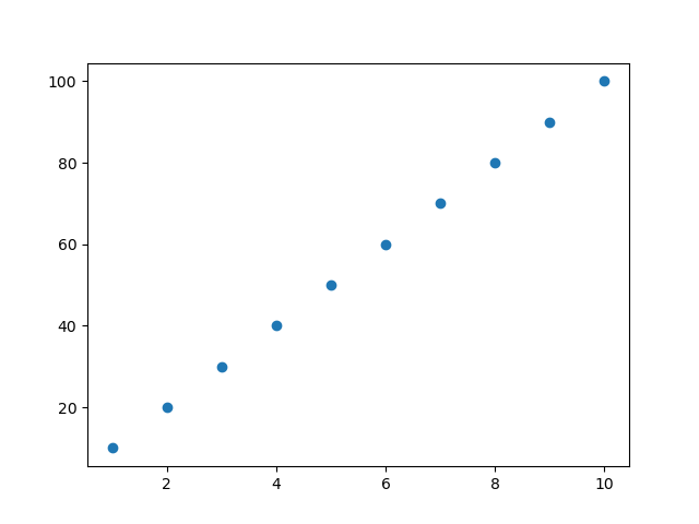
- The above code performs the following steps:
- First, it imports the necessary library: matplotlib.pyplot for plotting.
- Sample data for roll numbers and corresponding marks are defined in two lists: rollno and marks.
- The plt.scatter() function is used to create a scatter plot, with roll numbers on the x-axis and marks on the y-axis.
- Finally, plt.show() is called to display the plot.
- Now we will see how we can change the color of plotted points by using the color parameter passed into the scatter() function.
# Creating a scatter plot with green color
plt.scatter(rollno, marks, color='green')
plt.show()
- We can also change the marker style, which are the symbols used to represent data points. This can be done using the marker parameter. For example, we can use a star (*) as the marker.
# Creating a scatter plot with green color and star markers
plt.scatter(rollno, marks, color='green', marker='*')
plt.show()
- We can also increase the marker size using the markersize parameter.
# Creating a scatter plot with star markers of size 20
plt.scatter(rollno, marks, color='green', marker='*', s=100)
plt.show()
- xlabel and ylabel functions are used to set labels for the x-axis and y-axis respectively.
- The title function is used to set the title of the plot.
# Adding labels and title to the scatter plot
plt.scatter(rollno, marks, color='green', marker='*', s=100)
plt.xlabel('Roll Number')
plt.ylabel('Marks')
plt.title('Marks Distribution')
plt.show()
Output:
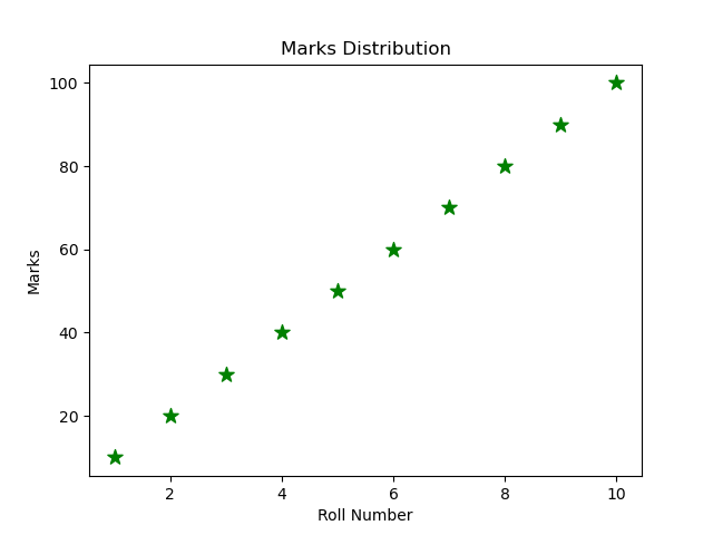
We can also work with data from a CSV file. For example:
import pandas as pd
import matplotlib.pyplot as plt

# Reading data from a CSV file
df = pd.read_csv('data.csv')

# Creating a scatter plot using data from the CSV file
plt.scatter(df['Roll No'], df['Marks'], color='blue', marker='o', s=50)
plt.xlabel('Roll Number')
plt.ylabel('Marks')
plt.title('Marks Distribution from CSV')
plt.show()
Line Plot
- A line plot is a type of chart that displays information as a series of data points called 'markers' connected by straight line segments.
- We use the plot() function from the pyplot module in Matplotlib to create line plots.
import matplotlib.pyplot as plt

# Sample data
rollno = [1, 2, 3, 4, 5, 6, 7, 8, 9, 10]
marks = [10, 20, 30, 40, 50, 60, 70, 80, 90, 100]

# Creating a simple line plot
plt.plot(rollno, marks)
plt.show()
Output:
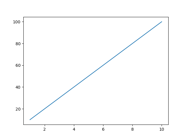
- Just like in scatter plots, we can change the color of the line using the color parameter.
- We can also add markers to the line plot using the marker parameter.
# Creating a line plot with red color and circle markers
plt.plot(rollno, marks, color='red', marker='o')
plt.show()
- We can change the line style using the linestyle parameter. Possible values
include:
- '-' for a solid line (default)
- '--' for a dashed line
- '-.' for a dash-dot line
- ':' for a dotted line
- We can adjust the line width using the linewidth parameter to make the line thicker or thinner.
# Creating a line plot with a dashed line style and specified line width
plt.plot(rollno, marks, color='red', linestyle='--', marker='o', linewidth=2)
plt.show()
- We can use the xlabel and ylabel functions to set labels for the x-axis and y-axis respectively, and the title function to set the title of the plot, just like in scatter plots.
# Adding labels and title to the line plot
plt.plot(rollno, marks, color='red', linestyle='--', marker='o')
plt.xlabel('Roll Number')
plt.ylabel('Marks')
plt.title('Marks Distribution')
plt.show()
Bar Graph
- A bar graph is a chart that presents categorical data with rectangular bars. The lengths of the bars are proportional to the values they represent.
- We use the bar() function from the pyplot module in Matplotlib to create bar graphs.
import matplotlib.pyplot as plt

# Sample data
categories = ['1-10', '11-20', '21-30', '31-40', '41-50']
values = [10, 20, 30, 40, 50]

# Creating a simple bar graph
plt.bar(categories, values)
plt.show()
Output:
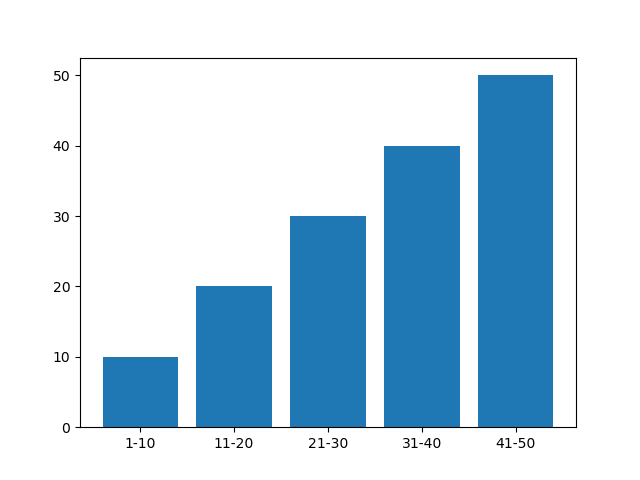
- Just like in scatter plots and line plots, we can change the color of the bars using the color parameter.
# Creating a bar graph with green bars
plt.bar(categories, values, color='green')
plt.show()
- We can add labels to the x-axis and y-axis using the xlabel and ylabel functions, and set a title for the bar graph using the title function.
# Adding labels and title to the bar graph
plt.bar(categories, values, color='green')
plt.xlabel('Categories')
plt.ylabel('Values')
plt.title('Sample Bar Graph')
plt.show()
- We can also change the width of the bars using the width parameter.
# Creating a bar graph with specified bar width
plt.bar(categories, values, color='green', width=0.5)
plt.show()
Horizontal Bar Graph
- A horizontal bar graph is a chart that presents categorical data with horizontal rectangular bars. The lengths of the bars are proportional to the values they represent.
- We use the barh() function from the pyplot module in Matplotlib to create horizontal bar graphs.
import matplotlib.pyplot as plt

# Sample data
categories = ['1-10', '11-20', '21-30', '31-40', '41-50']
values = [10, 20, 30, 40, 50]

# Creating a simple horizontal bar graph
plt.barh(categories, values)
plt.show()
Output:
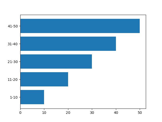
- Just like in scatter plots and line plots, we can change the color of the bars using the color parameter.
# Creating a horizontal bar graph with blue bars
plt.barh(categories, values, color='blue')
plt.show()
- We can add labels to the x-axis and y-axis using the xlabel and ylabel functions, and set a title for the bar graph using the title function.
# Adding labels and title to the horizontal bar graph
plt.barh(categories, values, color='blue')
plt.xlabel('Values')
plt.ylabel('Categories')
plt.title('Sample Horizontal Bar Graph')
plt.show()
- We can also change the width of the bars using the height parameter.
# Creating a horizontal bar graph with specified bar height
plt.barh(categories, values, color='blue', height=0.5)
plt.show()
Multiple Bar Chart with Matplotlib and NumPy
To draw multiple bar charts:
- Decide the number of X points using np.linspace() function based on the length of values in the sequence.
- Decide the thickness of each bar and adjust X points on the X-axis accordingly.
- Assign different colors to different data ranges.
- Keep the width constant for all ranges being plotted.
- Call plt.bar() for each data range to plot the bars.
Now let's break down the code and understand each part in detail:
import matplotlib.pyplot as plt
import numpy as np

# Sample data
a = [50, 60, 70, 80, 90]
b = [55, 65, 75, 85, 95]
x = np.linspace(1, 51, 5)

plt.bar(x, a, width=3, color='r', label='Australia')
plt.bar(x+3, b, width=3, color='g', label='India')

plt.xlabel('Overs')
plt.ylabel('Runs Scored')
plt.legend()
plt.show()
Output:
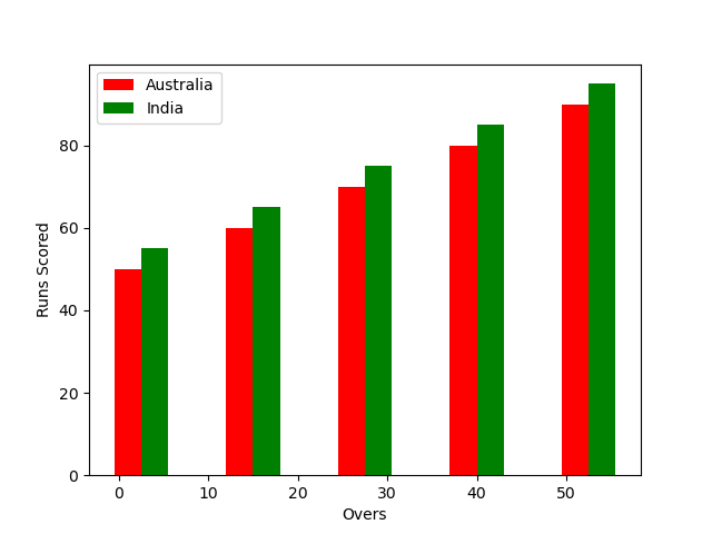
- import matplotlib.pyplot as plt: Imports the matplotlib library for plotting graphs and assigns it an alias plt.
- import numpy as np: Imports the numpy library for numerical computations and assigns it an alias np.
- a = [50, 60, 70, 80, 90]: Defines a list a containing values representing runs scored by a team (e.g., Australia) in different overs.
- b = [55, 65, 75, 85, 95]: Defines a list b containing values representing runs scored by another team (e.g., India) in the same overs.
- x = np.linspace(1, 51, 5): Creates an array x using np.linspace() function.
- The first parameter 1 is the starting point of the sequence.
- The second parameter 51 is the ending point of the sequence.
- The third parameter 5 is the number of points or steps in the sequence.
- np.linspace(1, 51, 5) generates 5 evenly spaced points starting from 1 and ending at 51.
- plt.bar(x, a, width=3, color='r', label='Australia'): Plots a bar chart for team Australia.
- x: Represents the x-axis values, which are the positions of the bars on the plot. These are the evenly spaced points generated by np.linspace().
- a: Represents the y-axis values, which are the heights of the bars, i.e., the runs scored by Australia.
- width=3: Specifies the width of each bar in the plot.
- color='r': Sets the color of the bars to red ('r').
- label='Australia': Adds a label for the data series, which will be used in the legend.
- plt.bar(x+3, b, width=3, color='g', label='India'): Plots another set of bars for team India.
- x+3: Shifts the x-axis positions by 3 units to the right, so that the bars for India are displayed next to the bars for Australia.
- b: Represents the y-axis values for India (runs scored).
- width=3: Specifies the width of each bar.
- color='g': Sets the color of the bars to green ('g').
- label='India': Adds a label for this data series in the legend.
- plt.xlabel('Overs'): Adds a label 'Overs' to the x-axis.
- plt.ylabel('Runs Scored'): Adds a label 'Runs Scored' to the y-axis. on
- plt.legend(): Displays the legend on the plot, which shows the labels ('Australia' and 'India') corresponding to the data series.
- plt.show(): Displays the plot with the bar chart, x-axis labeled as 'Overs', y-axis labeled as 'Runs Scored', and a legend showing the data series for Australia and India.
Pie Chart with Matplotlib
To create a pie chart using Matplotlib:
- Define the data to be represented in the pie chart.
- Call plt.pie() with the data to plot the pie chart.
- Customize the chart as needed, such as adding labels and colors.
- Display the chart using plt.show().
Now let's break down the code and understand each part:
import matplotlib.pyplot as plt

# Sample data
sizes = [30, 20, 15, 35]
labels = ['A', 'B', 'C', 'D']
colors = ['gold', 'lightcoral', 'lightskyblue', 'lightgreen']

plt.pie(sizes, labels=labels, colors=colors, autopct='%1.1f%%', startangle=140)
plt.axis('equal')  # Equal aspect ratio ensures that pie is drawn as a circle.
plt.title('Pie Chart Example')
plt.show()
Output:
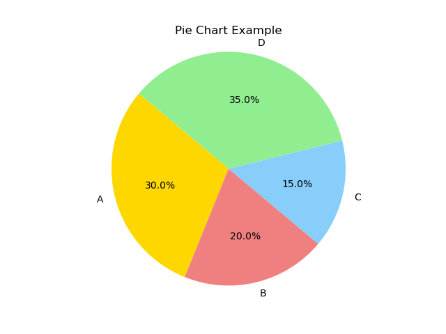
- import matplotlib.pyplot as plt: Imports the matplotlib library for plotting graphs and assigns it an alias plt.
- sizes = [30, 20, 15, 35]: Defines a list sizes representing the sizes or proportions of different data segments in the pie chart.
- labels = ['A', 'B', 'C', 'D']: Defines a list labels containing labels for each data segment.
- colors = ['gold', 'lightcoral', 'lightskyblue', 'lightgreen']: Defines a list colors specifying colors for each data segment.
- plt.pie(sizes, labels=labels, colors=colors, autopct='%1.1f%%', startangle=140): Creates the pie chart.
- sizes: Specifies the sizes or proportions of the pie chart segments.
- labels=labels: Adds labels to each segment based on the labels list.
- colors=colors: Sets colors for each segment based on the colors list.
- autopct='%1.1f%%': Displays the percentage of each segment in the chart with one decimal place.
- startangle=140: Specifies the starting angle for the first segment of the pie chart (optional).
- plt.axis('equal'): Ensures that the pie chart is drawn as a circle by setting equal aspect ratio.
- plt.title('Pie Chart Example'): Adds a title to the pie chart.
- plt.show(): Displays the pie chart.
Histogram: A Visualization of Data Distribution
A histogram is a type of bar chart that represents the distribution of numerical data. It divides data into intervals called bins and displays the frequency of data points falling into each bin.
- plt.hist(): The plt.hist() function is used to create a histogram in Matplotlib.
- Data Distribution: Histograms are useful for visualizing the distribution of data, such as whether it is normally distributed, skewed, or has outliers.
- Bins: Bins are intervals into which data is divided. The number of bins and their width can be adjusted to visualize the data more effectively.
- Frequency: The height of each bar in a histogram represents the frequency of data points in that bin.
Here's an example code for creating a histogram:
import matplotlib.pyplot as plt
import numpy as np

# Generate random data
np.random.seed(0)
data = np.random.randn(1000)

plt.hist(data, bins=30, color='blue', alpha=0.7)
plt.xlabel('Value')
plt.ylabel('Frequency')
plt.title('Histogram Example')
plt.show()
Output:
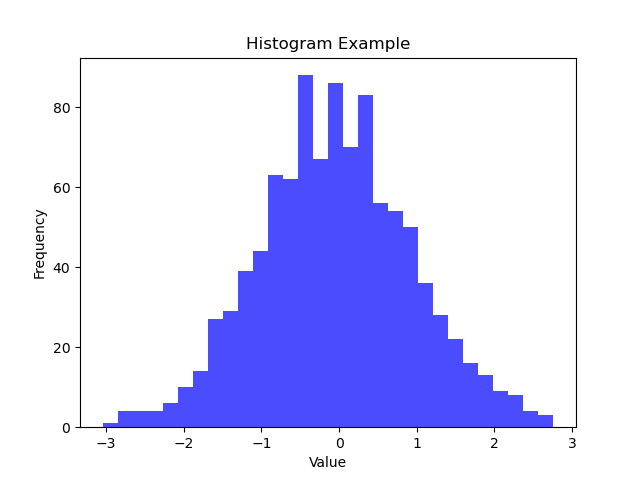
- import matplotlib.pyplot as plt: Imports the Matplotlib library for plotting graphs.
- import numpy as np: Imports the NumPy library for numerical computations.
- np.random.seed(0): Sets the random seed for reproducibility of random data.
- data = np.random.randn(1000): Generates 1000 random data points using a normal distribution (mean=0, standard deviation=1).
- plt.hist(data, bins=30, color='blue', alpha=0.7): Creates a histogram with 30 bins, blue bars, and transparency set to 0.7 (alpha=0.7).
- plt.xlabel('Value'): Adds a label 'Value' to the x-axis.
- plt.ylabel('Frequency'): Adds a label 'Frequency' to the y-axis.
- plt.title('Histogram Example'): Adds a title to the histogram.
- plt.show(): Displays the histogram plot.
Multiple Box Plots for Different Data Sets
Here's an example of creating multiple box plots for three different data sets:
import matplotlib.pyplot as plt

# Predefined data sets
data1 = [10, 20, 30, 40, 50]
data2 = [15, 25, 35, 45, 55]
data3 = [5, 15, 25, 35, 45]

plt.boxplot([data1, data2, data3], labels=['Data 1', 'Data 2', 'Data 3'])
plt.xlabel('Data Sets')
plt.ylabel('Values')
plt.title('Multiple Box Plots Example')
plt.show()
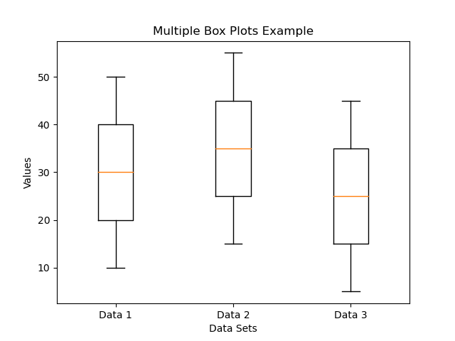
- import matplotlib.pyplot as plt: Imports Matplotlib for plotting.
- data1, data2, data3: Predefined data sets for the box plots.
- plt.boxplot([data1, data2, data3], labels=['Data 1', 'Data 2', 'Data 3']): Creates multiple box plots for the three data sets with labels.
- plt.xlabel('Data Sets'): Adds a label 'Data Sets' to the x-axis.
- plt.ylabel('Values'): Adds a label 'Values' to the y-axis.
- plt.title('Multiple Box Plots Example'): Adds a title to the plot.
- plt.show(): Displays the box plots.
Types of Graphs and When to Use Them
- Scatter Plot: A scatter plot is a type of plot that displays data points as markers in a
two-dimensional space,
typically to observe the relationship between two variables.
- When to use: Use scatter plots to visualize the relationship or correlation between two continuous variables, such as height vs. weight or temperature vs. time.
- Line Plot: A line plot is a type of plot that displays data points connected by straight lines,
typically to
show
trends over time or ordered data points.
- When to use: Use line plots to display trends or changes over time, such as stock prices, temperature changes, or sales data over months.
- Bar Graph: A bar graph is a type of plot that represents data with rectangular bars, where the
length or height
of
each bar is proportional to the value it represents.
- When to use: Use bar graphs to compare different categories or groups, such as the sales of different products, population by region, or scores of different students.
- Horizontal Bar Graph: A horizontal bar graph is similar to a bar graph, but the bars are
displayed horizontally instead of
vertically.
- When to use: Use horizontal bar graphs when you have long category names or when comparing a small number of categories.
- Multiple Bar Graph: A multiple bar graph displays multiple sets of data side by side for
comparison,
using groups of
rectangular bars.
- When to use: Use multiple bar graphs to compare multiple sets of data across the same categories, such as comparing sales of different products across multiple years.
- Pie Chart:
A pie chart is a circular graph divided into sectors, where each sector represents a proportion
of
the
whole.
- When to use: Use pie charts to show the relative proportions or percentages of a whole, such as market share distribution, survey results, or budget allocation.
- Histogram:
A histogram is a type of plot that displays the distribution of a dataset by grouping data into
bins
and
showing the frequency of data points in each bin.
- When to use: Use histograms to visualize the distribution of a dataset, such as the frequency of exam scores, age distribution, or the distribution of income levels.
- 8. Box Plot:
A box plot, also known as a box-and-whisker plot, is a type of plot that displays the
distribution
of
a
dataset through five summary statistics: minimum, first quartile (Q1), median, third quartile
(Q3),
and
maximum.
- When to use: Use box plots to visualize the distribution, variability, and outliers of a dataset, such as comparing test scores, salaries, or experiment results across different groups.