Computing
Before diving into soft computing, it's essential to first understand what computing is and familiarize ourselves with the core terminologies related to computing.
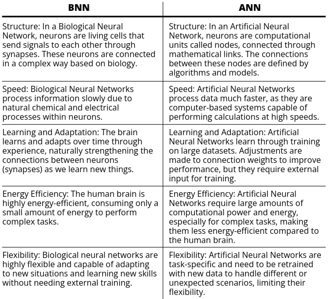
- The following diagram represents the basic process that occurs in computing:
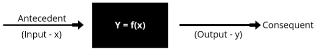
- In this diagram, we observe that there is a function, f, which takes some input, x, and produces an output, y. The input is referred to as the Antecedent, while the output is called the Consequent.
- The function f can also be called a formal method, algorithm, or a mapping function. It represents the logic or steps used to process the input and generate the output.
- The middle part of this diagram is known as the computing unit, where the function resides. This is where we feed the input, and a process occurs to convert that input into the desired output y.
- In the computing process, the steps that guide how the input is manipulated are called control actions. These control actions ensure that the input gradually approaches the desired output. The moment the process completes, we obtain the final result, known as the Consequent.
- Basic Characteristics Related to Computing:
- Precise Solution: Computing is used to produce a solution that is exact and definitive.
- Unambiguous & Accurate: The control actions within the computing unit must be unambiguous, meaning they must have only one interpretation. Each control action should also be accurate to ensure that the process is valid and reliable.
- Mathematical Model: A well-defined algorithm is a requirement for solving any problem through computing. This algorithm is essentially a mathematical model that represents the problem and its solution process.
- In computing, there are two main types:
- Hard Computing
- Soft Computing
Hard Computing
- Hard computing refers to a traditional computing approach where the results are always precise and exact. This is because hard computing relies on well-defined mathematical models and algorithms to solve problems. There is no room for approximation, as every calculation or action leads to a deterministic output.
- Main Features of Hard Computing:
- Exact Results: The results in hard computing are always exact. This means, whenever we solve a problem using hard computing methods, the answer will always be the same and correct. There is no room for uncertainty or approximation.
- Clear Control Actions: In hard computing, the steps or actions we take to solve a problem are clear and have only one meaning. For example, when following an algorithm, each step must be clearly understood and should only have one possible result. There should be no confusion or multiple meanings for a single step. This is called being "unambiguous."
- Based on Mathematical Models: All the actions in hard computing are based on well-defined mathematical rules or formulas. This means that each step we take while solving a problem has a proper mathematical explanation behind it. These steps follow a fixed pattern or method, which helps in solving the problem in a precise way.
- Examples of Hard Computing:
- Numerical Problems: Problems that require accurate mathematical calculations, like solving equations or doing arithmetic, are examples of hard computing.
- Searching and Sorting Algorithms: In computer science, methods like searching for an item in a list or sorting a list in a particular order are solved using hard computing techniques because they always give an exact answer.
- Computational Geometry Problems: These are problems related to shapes, distances, and areas in geometry. For example, calculating the shortest distance between two points or finding the area of a triangle requires exact methods, which is where hard computing comes in.
Soft Computing
- Soft Computing is an approach to computing that models the human mind’s ability to make decisions in an uncertain, imprecise, or complex environment. Unlike traditional, or "hard," computing, which relies on exact, binary logic (0s and 1s), soft computing deals with approximation, flexibility, and learning from experience to solve complex real-world problems.
- Soft computing techniques focus on developing systems that can handle ambiguity, uncertainty, and approximation, making them well-suited for fields like artificial intelligence (AI), pattern recognition, and robotics.
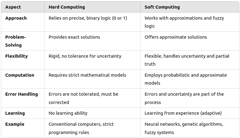
Difference between Hard and Soft Computing
Requirement of Soft Computing
Soft computing is essential because many real-world problems are too complex for traditional computing methods. Systems must handle:
- Uncertainty: Data may not always be precise, requiring flexible models.
- Partial truths: Situations where a simple binary "true/false" answer isn’t sufficient.
- Imprecision: Many problems, such as human language processing, involve vague or imprecise inputs.
- Complex systems: Soft computing helps in dealing with complex, non-linear systems, like weather prediction or stock market analysis.
Importance of Soft Computing
- Handles Uncertainty and Approximation:
- Traditional algorithms often require exact inputs, but real-world problems don't always have precise data. Soft computing methods can handle uncertainty, making them more suitable for practical applications.
- Example: In medical diagnosis, data such as symptoms might be uncertain or incomplete, and soft computing helps make decisions despite that.
- Flexible and Adaptive:
- Soft computing systems are highly adaptive to changes and can learn from new data. This makes them ideal for dynamic environments where conditions or inputs change over time.
- Example: In stock market predictions, a neural network can learn from past trends and adapt to new market conditions.
- Tolerance to Noise and Incompleteness:
- Soft computing techniques can work with noisy data (data that is random or disturbed) and incomplete information. They don’t require the exact and clean data that traditional methods do.
- Example: Image recognition systems in self-driving cars can still work even when the images are slightly unclear or distorted.
- Ease of Implementation:
- Soft computing techniques like fuzzy logic and genetic algorithms are often easier to implement for complex, real-world problems compared to traditional methods. They don’t require a precise model of the system but instead learn from examples.
- Example: In control systems, fuzzy logic can be quickly applied to model human-like decision-making without needing complex mathematical models.
- Incorporates Human-Like Reasoning:
- Soft computing allows for reasoning based on approximate data, mimicking human decision-making. This is especially useful in applications where exact answers aren’t available.
- Example: In customer service, fuzzy logic can simulate human-like reasoning in responding to customer queries.
Various Techniques of Soft Computing
- Fuzzy Logic: Mimics human reasoning, allowing for more than just "true" or "false" outcomes. It’s widely used in control systems, such as thermostats or automated vehicle systems.
- Neural Networks: Modeled after the human brain, these networks learn from data and improve over time. They are used in areas like image recognition, speech processing, and autonomous systems.
- Genetic Algorithms: Inspired by natural selection, these algorithms "evolve" solutions over generations. They are useful for optimization problems, such as route planning or complex decision-making.
- Probabilistic Reasoning: Deals with uncertainty using probabilities. It is useful in situations where outcomes are not deterministic, like predicting stock market trends or diagnosing diseases.
Applications of Soft Computing
Soft computing techniques are applied in a variety of fields, including:
- Artificial Intelligence (AI): Many AI systems rely on neural networks and fuzzy logic to emulate human decision-making.
- Pattern Recognition: Soft computing helps identify patterns in complex data, such as handwriting recognition or facial recognition.
- Robotics: Soft computing enables robots to navigate environments with uncertain data, making them more adaptable.
- Data Mining: Soft computing techniques are used to discover patterns and relationships in large datasets.
- Control Systems: Fuzzy logic controllers are used in industrial systems, like temperature control in manufacturing plants.
- Medicine: Soft computing helps in diagnosing diseases, predicting patient outcomes, and optimizing treatment plans.
- Economics and Finance: Used in predicting market trends, risk analysis, and portfolio optimization.
Fundamentals of ANN
Artificial Neural Networks (ANNs) are a key component of modern artificial intelligence, inspired by the way biological neural networks in the human brain function. ANNs are designed to mimic the brain's ability to process information, learn from data, and make decisions. This section explores the fundamentals of ANNs, starting with an understanding of biological neural networks, which serve as the foundation for developing these sophisticated computational models. By examining how neurons interact in the human brain, we can better appreciate how artificial networks are structured and how they perform various tasks.
Biological Neural Network
- First, we should understand that a neural network is a massive collection of neurons that are interconnected with one another.
- The human brain contains billions of neurons, approximately 1013, and all these neurons are interconnected to form a complex network.
- The following is a diagram of a single biological neuron:
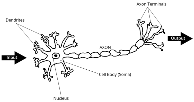
- A biological neuron consists of dendrites, which are responsible for collecting inputs. Inside the neuron, there is a cell body (also known as the soma), and within the cell body, we find the nucleus. The dendrites collect the input signals, and the cell body processes that input. Once processed, the output is transferred via the axon. The axon is the part of the neuron that carries the output signals to other neurons.
- In the human brain, we have billions of neurons, and the dendrites of one neuron connect with the axons of other neurons. The point where two neurons connect is called a synapse. Information is stored and transferred across these synapses. As we store more information in our brains, the synapses strengthen, allowing us to retain that information. With billions of neurons, we also have billions of synapses, which play a key role in memory and learning.
- For example, when we read a question in an exam, the information is sent to our brain through neurons. Another example is when a mosquito bites us; the signal of pain is sent to our brain, and we respond to it through neural signals.
- Definition of Biological Neural Network: A biological neural network is a network of neurons that processes and transmits information in the brain. It is the basis of how humans think, learn, and make decisions. The neurons communicate with each other through synapses, which strengthen as we store more information, allowing us to retain and recall data.
- The development of Artificial Neural Networks (ANNs) was inspired by biological neural networks (BNNs). Researchers, observing how the human brain is capable of understanding questions, thinking, and making decisions without any external control, started studying BNNs closely. They wanted to replicate this ability in machines.
- This is how the concept of artificial neural networks (ANNs) was born. Researchers aimed to build machines that could think and act like humans, think rationally, and perform tasks without human intervention. The structure and function of ANNs are modeled on biological neural networks, which is why BNNs played a significant role in the development of ANNs.
Artificial Neural Network
- An Artificial Neural Network (ANN) is designed to develop a computational system that models the human brain. This model allows ANNs to perform a variety of tasks more efficiently than traditional computer systems. For example, while traditional computers might take a long time to perform a task, an ANN can complete the same task in a much shorter period. ANNs are used for various applications such as classification, pattern recognition, and optimization. Essentially, ANNs are developed to mimic the functionality of the human brain and perform tasks faster and more efficiently than conventional systems.
- The main objective of an ANN is to process and analyze data in a manner similar to how the human brain does, allowing it to make decisions, recognize patterns, and solve complex problems with speed and accuracy.
- We can also describe an ANN as an efficient information processing system that resembles the characteristics of a biological neural network. ANNs are designed to process information in a way that is similar to how the brain processes information.
- An ANN consists of highly interconnected processing elements known as nodes. In the human brain, these processing elements are neurons. Similarly, in ANNs, nodes act like neurons and are interconnected with each other through links. Each node receives inputs, processes them, and sends outputs to other nodes. This network of nodes and connections allows ANNs to perform complex tasks by processing information in a distributed manner.
- For example, consider an ANN with two input nodes (A and B) connected to one output node (C).
Node A is connected to node C, and node B is also connected to node C. Suppose node A receives
an input signal called x1 and node B receives an input signal called x2. The output node C will
receive a combined signal y. We assign weights to the connections between the nodes: w1 for the
connection between A and C, and w2 for the connection between B and C.
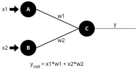
The weights are crucial because they determine the strength and importance of each input signal. By adjusting the weights, the ANN can learn which inputs are more significant for making accurate predictions or decisions. The net input to node C is calculated as follows:
Net Input = x1 * w1 + x2 * w2
This calculation provides the net input to node C, but to determine the actual output, we need to apply an activation function to the net input. The activation function helps to decide whether the neuron should be activated or not. After applying the activation function, we get the final output for node C.
This example illustrates a simple ANN structure. In more complex ANNs, there can be multiple input nodes (A, B, C, D, E, F), each with its own input signals (x1, x2, x3, x4, x5, etc.) and weights (w1, w2, etc.). The net input to the output node is calculated similarly, but with many more inputs and weights. The final output is determined after applying the activation function to the net input.
Difference between ANN and BNN
Artificial Neural Networks (ANNs) and Biological Neural Networks (BNNs) are both networks of neurons, but they function differently. While BNNs exist naturally in the human brain, ANNs are man-made systems created to mimic the brain's functioning. In this section, we’ll explore the key differences between these two types of neural networks.
Building Blocks of Artificial Neural Networks (ANN)
To understand Artificial Neural Networks (ANN), we must first examine its foundational components. Just like any structure, a neural network is built upon certain key elements that define how it processes information, learns from data, and makes predictions.
1: Architecture of ANN
Architecture refers to the layout or structure of an ANN. It is how the neurons (units) are organized in layers and how these layers are connected to each other.
- Layers: An ANN typically consists of three types of layers:
- Input Layer: Receives the raw data (like images, numbers, etc.) and passes it on to the next layer.
- Hidden Layer(s): These layers process the input and extract patterns. The number of hidden layers and neurons in each layer can vary.
- Output Layer: Provides the final result (e.g., a classification label or prediction).
Input Layer       Hidden Layer       Output Layer
    o                  o                    o
    | \              / | \                / |
    |  \            /  |  \              /  |
    o---o----------o---o---o------------o   o
    |  / \        / \  |  / \          /    |
    | /   \      /   \ | /   \        /     |
    o      \    /      o      \      /      o
            \  /               \    /
             o------------------o--o
The architecture of a neural network defines how data flows through the network, from input to output, and how decisions are made at each step.
- Connection with Weights: The architecture alone does not make the network functional. The magic happens when we assign weights to the connections between neurons. These weights determine the strength and impact of each connection on the final output.
2: Setting of Weights
Weights are numerical values that control how much influence one neuron has over another. Every connection between neurons has a weight associated with it, and these weights are learned during the training process.
- Initial Weights: At the start, weights are usually assigned randomly. These weights are adjusted as the network learns from the data.
- Role of Weights: The higher the weight between two neurons, the stronger the connection, meaning the output from one neuron has a greater influence on the next neuron’s decision.
- Learning: During training, the network adjusts the weights to minimize errors in its predictions. This process is called training the network, and it’s essential for the network’s ability to learn from data.
Connection with Activation Functions: Once the weights determine how much influence one neuron’s output has, we need a mechanism to decide whether this output should be passed forward or "activated." That’s where activation functions come in.
3: Activation Functions
An activation function is a mathematical function that determines whether a neuron should be activated (fired) based on the weighted sum of its inputs. It introduces non-linearity to the network, allowing it to solve complex problems.
- Importance of activation function: let us assume a person is performing some task. To make the task more efficient and to obtain correct results, some force or motivation may be given. This force or motivation helps in achieving the correct results. In a similar way, the activation function is applied over the net input of the network to calculate the output of an ANN so that we get a better output or result.
Now we will discuss each of the activation functions one by one:
1: Identity Function
- Also known as the linear function because the output is identical to the input.
- It can be defined as:
f(x) = x for all x.
Here, if the net input is x, then the output will also be x.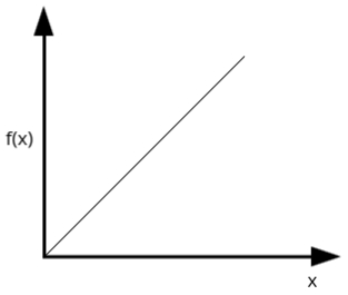
- The input layer often uses the identity activation function because no transformation is needed.
2: Binary Step Function
- This function can be defined as:
\( f(x) = \begin{cases} 1 & \text{if } x \geq \theta \\ 0 & \text{if } x < \theta \end{cases} \)
where θ is the threshold value. If the net input (x) is greater than or equal to this threshold value, the output is 1, otherwise, it is 0.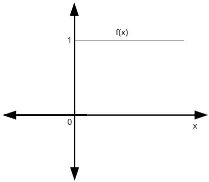
- It is widely used in single-layer neural networks where the output needs to be binary (either 0 or 1).
3: Bipolar Step Function
- Similar to the binary step function, but it outputs either +1 or -1 instead of 1 or 0.
- It can be defined as:
\( f(x) = \begin{cases} 1 & \text{if } x \geq \theta \\ -1 & \text{if } x < \theta \end{cases} \)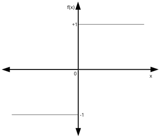
- Used when outputs are expected to be in the range of +1 and -1, often in single-layer networks.
4: Sigmoidal Activation Functions
Sigmoidal functions introduce non-linearity to the network and are widely used in backpropagation-based neural networks. There are two main types:
a) Binary Sigmoidal Function (Logistic Function)
- It can be defined as:
\( f(x) = \frac{1}{1 + e^{-\lambda x}} \)
where λ (lambda) is the steepness parameter, and x is the net input. - The output of the binary sigmoidal function is always between 0 and 1.
- This function has a peculiar property: its derivative is:
\( f'(x) = \lambda f(x) (1 - f(x)) \)
b) Bipolar Sigmoidal Function
- It can be defined as:
\( f(x) = \frac{2}{1 + e^{-\lambda x}} - 1 \)
where λ (lambda) is the steepness parameter, and x is the net input. - The output of the bipolar sigmoidal function ranges from -1 to +1.
- Its derivative is:
\( f'(x) = \frac{\lambda}{2} (1 + f(x)) (1 - f(x)) \)
5: Ramp Activation Function
- This function is a combination of step and linear functions.
- It can be defined as:
\( f(x) = \begin{cases} 1 & \text{if } x > 1 \\ 0 & \text{if } x < 0 \\ x & \text{if } 0 \leq x \leq 1 \end{cases} \)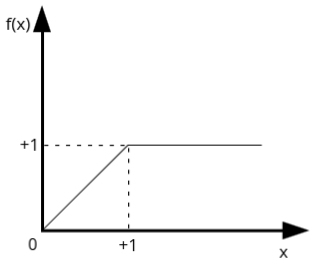
- It outputs 0 for inputs less than 0, increases linearly with inputs between 0 and 1, and outputs 1 for inputs greater than 1.
Activation functions play a vital role in artificial neural networks by introducing non-linearity and helping the network learn complex patterns.
Sigmoid Activation Function Solved Example
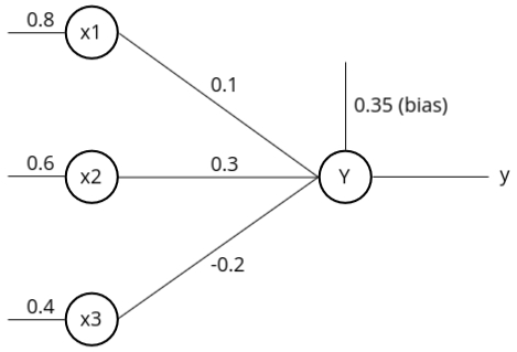
In this case, we have a neural network with an input layer and an output layer. The input layer has three neurons, and the output layer has one neuron. The inputs are \(0.8\), \(0.6\), and \(0.4\). The bias weight is \(0.35\). The weights associated with the three neurons are \(0.1\), \(0.3\), and \(-0.2\).
There are two types of sigmoid functions:
- Binary Sigmoid Activation Function: The equation is \(y = F(y_n) = \frac{1}{1 + e^{-y_n}}\) where \(y_n\) is the net input to that particular neuron.
- Bipolar Sigmoid Activation Function: The equation is \(y = F(y_n) = \frac{2}{1 + e^{-y_n}} - 1\) where again we need to know the net input \(y_n\).
To calculate the net input \(y_n\), we find the sum of the product of the inputs and weights. The equation looks like this:
\(y_n = B + \sum_{i=1}^{n} (x_i \cdot w_i)\)In this case, \(n\) is the number of input neurons, which is 3.
Expanding the equation:
\(y_n = B + (x_1 \cdot w_1) + (x_2 \cdot w_2) + (x_3 \cdot w_3)\)Substituting the values:
- Bias (\(B\)) = \(0.35\)
- \(x_1 = 0.8, \, w_1 = 0.1\)
- \(x_2 = 0.6, \, w_2 = 0.3\)
- \(x_3 = 0.4, \, w_3 = -0.2\)
Now solving the equation:
\(y_n = 0.35 + (0.8 \cdot 0.1) + (0.6 \cdot 0.3) + (0.4 \cdot -0.2)\)After calculation, we get \(y_n = 0.53\) as the net input to the neuron.
Now we can use this net input to find the outputs:
- Binary Sigmoid Activation Function: Using the net input in the binary sigmoid equation, we get: \( \text{output} = \frac{1}{1 + e^{-0.53}} \approx 0.628\)
- Bipolar Sigmoid Activation Function: Using the net input in the bipolar sigmoid equation, we get: \( \text{output} = \frac{2}{1 + e^{-0.53}} - 1 \approx 0.257\)
McCulloch-Pitts Neuron
The McCulloch-Pitts (MP) neuron, introduced in 1943 by Warren McCulloch and Walter Pitts, is one of the earliest models of artificial neural networks. This pioneering work laid the foundation for the field of neural computing and artificial intelligence. The MP neuron was designed to mimic the functioning of biological neurons in the human brain, aiming to represent logical operations in a simplified manner. Unlike more complex models, the MP neuron operates based on binary inputs and outputs, effectively simulating the way neurons fire in response to stimuli. As such, it serves as a fundamental building block in understanding neural networks and provides insights into how information processing occurs within more sophisticated models. This model is crucial for grasping essential concepts in neural networks, including activation functions, thresholds, and the basic principles of learning.
Architecture of McCulloch-Pitts Neuron
The architecture of the MP neuron consists of two layers:
- Input Layer: Contains the input neurons.
- Output Layer: Contains the output neuron.
The input layer neurons are connected to the output neuron through directed edges, which can have either positive or negative weights. Positive weights are associated with excitatory nodes, while negative weights are associated with inhibitory nodes.
Activation Function and Threshold Value
The firing of the output neuron depends on a threshold value. The activation function of this network can be defined as follows:
Let \(F(y_n)\) be the activation function, where \(y_n\) is the net input. The function can be expressed as:
\(F(y_n) = \begin{cases} 1 & \text{if } y_n \geq θ \\ 0 & \text{otherwise} \end{cases}\)
Here, θ is the threshold value. For the neuron to fire, the net input \(y_n\) must be greater than or equal to the threshold value.
Determining the Threshold Value
The value of θ should be greater than \(n \cdot W - P\), where:
- \(n\) = Number of neurons in the input layer
- \(W\) = Positive weight
- \(P\) = Negative weight
AND Function Implementation Using McCulloch-Pitts Neuron
1. Truth Table of AND Function
The truth table for the AND function clearly illustrates the relationship between the inputs and the output. In the context of logic gates, an AND gate outputs a high signal (1) only when all its inputs are high. This behavior is fundamental in digital electronics and can be represented as follows:
+---------+---------+--------+
| Input X1| Input X2| Output |
+---------+---------+--------+
|    0    |    0    |   0    |
|    0    |    1    |   0    |
|    1    |    0    |   0    |
|    1    |    1    |   1    |
+---------+---------+--------+
From the truth table, it is evident that the output is high only when both inputs are high (1). If either input is low (0), the output is also low (0). This binary relationship forms the basis of how the McCulloch-Pitts neuron will function in this scenario.
2. Understanding Weights and Threshold
One crucial aspect to note is that the McCulloch-Pitts neuron does not utilize a built-in training algorithm like modern neural networks. Instead, we must manually analyze the input combinations to determine the optimal weights and threshold values required for the desired output behavior.
For implementing the AND function, we can assume the following weights for our inputs:
- \(W_1 = 1\)
- \(W_2 = 1\)
These weights represent the contribution of each input to the net input of the neuron. With these assumptions in place, we can now calculate the net input at the output neuron based on various input combinations:
Net Input Calculations
Let’s compute the net input \(y_n\) for each possible combination of inputs:
1. For inputs \(X_1 = 1\) and \(X_2 = 1\):
\(y_n = (X_1 \cdot W_1) + (X_2 \cdot W_2) = (1 \cdot 1) + (1 \cdot 1) = 2\)
In this scenario, both inputs are high, resulting in a net input of 2.
2. For inputs \(X_1 = 1\) and \(X_2 = 0\):
\(y_n = (1 \cdot 1) + (0 \cdot 1) = 1\)
Here, the first input is high while the second is low, yielding a net input of 1.
3. For inputs \(X_1 = 0\) and \(X_2 = 1\):
\(y_n = (0 \cdot 1) + (1 \cdot 1) = 1\)
Similar to the previous case, only one input is high, resulting in a net input of 1.
4. For inputs \(X_1 = 0\) and \(X_2 = 0\):
\(y_n = (0 \cdot 1) + (0 \cdot 1) = 0\)
Both inputs being low produces a net input of 0, indicating that the neuron does not fire.
3. Determining the Threshold Value
To ensure that the McCulloch-Pitts neuron fires (outputs 1) only when both inputs are high (1), we need to establish an appropriate threshold value, denoted as \(\theta\). Based on our previous calculations, we can conclude:
- If \(\theta \geq 2\), the neuron will fire when both inputs are high (1).
- If \(\theta < 2\), the neuron will not fire in cases where either input is low (0).
Thus, we determine that the threshold value \(\theta\) should be set to 2 to achieve the desired behavior of the AND function.
Additionally, we can calculate the threshold value using the following equation:
\(\theta \geq n \cdot W - P\)
Where:
- \(n\) is the number of neurons in the input layer (in this case, \(n = 2\)).
- \(W\) is the positive weight (here, \(W = 1\)).
- \(P\) is the negative weight, which in this case is \(0\) since we do not have inhibitory inputs.
Substituting these values into the equation gives:
\(\theta \geq 2 \cdot 1 - 0 = 2\)
Thus, both methods confirm that the threshold value should be set to 2.
4. Final Activation Function
The final activation function for the McCulloch-Pitts neuron can be expressed mathematically as:
\(F(y_n) = \begin{cases} 1 & \text{if } y_n \geq 2 \\ 0 & \text{otherwise} \end{cases}\)
This function confirms that the neuron will fire (output 1) only when both inputs \(X_1\) and \(X_2\) are equal to 1, effectively implementing the AND logical function. The simplicity of the McCulloch-Pitts model highlights its significance as a foundational concept in neural network theory, paving the way for more complex learning algorithms and structures in modern artificial intelligence.
ANDNOT Function Implementation Using McCulloch-Pitts Neuron
1. Truth Table of ANDNOT Function
The truth table for the ANDNOT function clearly illustrates the relationship between the inputs and the output. In this case, we have two inputs: \(X_1\) and \(X_2\), and \(Y\) is the output. The ANDNOT function outputs a high signal (1) only when \(X_1\) is high (1) and \(X_2\) is low (0). This behavior can be represented as follows:
+---------+---------+--------+
| Input X1| Input X2| Output |
+---------+---------+--------+
|    0    |    0    |   0    |
|    0    |    1    |   0    |
|    1    |    0    |   1    |
|    1    |    1    |   0    |
+---------+---------+--------+
From the truth table, it is evident that the output is high only when \(X_1\) is high (1) and \(X_2\) is low (0). In all other cases, the output is low (0). This binary relationship forms the basis of how the McCulloch-Pitts neuron will function in this scenario.
2. Understanding Weights and Threshold
One crucial aspect to note is that the McCulloch-Pitts neuron does not utilize a built-in training algorithm. Therefore, we need to analyze the input combinations to determine the optimal weights and threshold values required for the desired output behavior.
For implementing the ANDNOT function, we can assume the following weights for our inputs:
- \(W_1 = 1\)
- \(W_2 = -1\)
These weights indicate that the first input contributes positively to the net input, while the second input contributes negatively. With these assumptions in place, we can now calculate the net input at the output neuron based on various input combinations:
Net Input Calculations
Let’s compute the net input \(y_n\) for each possible combination of inputs:
1. For inputs \(X_1 = 1\) and \(X_2 = 1\):
\(y_n = (X_1 \cdot W_1) + (X_2 \cdot W_2) = (1 \cdot 1) + (1 \cdot -1) = 0\)
In this scenario, both inputs are high, resulting in a net input of 0.
2. For inputs \(X_1 = 1\) and \(X_2 = 0\):
\(y_n = (1 \cdot 1) + (0 \cdot -1) = 1\)
Here, the first input is high while the second is low, yielding a net input of 1.
3. For inputs \(X_1 = 0\) and \(X_2 = 1\):
\(y_n = (0 \cdot 1) + (1 \cdot -1) = -1\)
In this case, only the second input is high, resulting in a negative net input of -1.
4. For inputs \(X_1 = 0\) and \(X_2 = 0\):
\(y_n = (0 \cdot 1) + (0 \cdot -1) = 0\)
Both inputs being low produces a net input of 0, indicating that the neuron does not fire.
3. Determining the Threshold Value
To ensure that the McCulloch-Pitts neuron fires (outputs 1) only when \(X_1\) is high (1) and \(X_2\) is low (0), we need to establish an appropriate threshold value, denoted as \(\theta\). Based on our previous calculations, we can conclude:
- If \(\theta \leq 1\), the neuron will fire when \(X_1\) is 1 and \(X_2\) is 0.
- If \(\theta > 1\), the neuron will not fire in cases where \(X_2\) is high (1).
Thus, we determine that the threshold value \(\theta\) should be set to 1 to achieve the desired behavior of the ANDNOT function.
Additionally, we can calculate the threshold value using the following equation:
\(\theta \geq n \cdot W - P\)
Where:
- \(n\) is the number of neurons in the input layer (in this case, \(n = 2\)).
- \(W\) is the positive weight (here, \(W = 1\)).
- \(P\) is the negative weight (in this case, \(P = 1\)).
Substituting these values into the equation gives:
\(\theta \geq 2 \cdot 1 - 1 = 1\)
Thus, both methods confirm that the threshold value should be set to 1.
4. Final Activation Function
The final activation function for the McCulloch-Pitts neuron can be expressed mathematically as:
\(F(y_n) = \begin{cases} 1 & \text{if } y_n \geq 1 \\ 0 & \text{otherwise} \end{cases}\)
This function confirms that the neuron will fire (output 1) only when \(X_1\) is equal to 1 and \(X_2\) is equal to 0, effectively implementing the ANDNOT logical function.
Hebb Network / Hebbian Rule
1. Introduction to Hebbian Rule
The Hebbian Rule is one of the simplest learning rules under artificial neural networks. It was introduced in 1949 by Donald Hebb. According to Hebb, learning in the brain occurs due to changes in the synaptic gap, which can be attributed to metabolic changes or growth. This rule is based on the biological processes that occur in the brain during learning.
To understand the Hebbian Rule, let’s first consider the structure of a biological neuron. Each neuron has three main parts:
- Cell Body (Soma): This is where the nucleus is located.
- Axon: A long connection extending from one neuron to another.
- Dendrites: Small nerves connected to the cell body that transmit electrical impulses.
The electrical impulses are passed from one neuron to another through synapses, which are small gaps between neurons. When learning occurs, metabolic changes happen in the synaptic gap, leading to the formation of new connections between neurons.
2. Hebbian Rule Definition
Donald Hebb's definition of the Hebbian Rule is as follows:
"When an axon of cell A is near enough to excite cell B and repeatedly or persistently fires it, some growth process or metabolic change takes place in one or both cells."
In simpler terms, if neuron A excites neuron B frequently, changes occur in their synaptic gap, which strengthens the connection between the two neurons.
Hebb's Rule was inspired by the way learning happens in the human brain. A relatable example of this can be seen when learning to drive. Initially, when you start driving, you are conscious of every action, like turning or reversing. However, over time, as it becomes a habit, you can drive effortlessly while doing other tasks, like listening to music. This example demonstrates how neurons become trained and perform tasks automatically over time, which is the core idea of Hebb’s learning theory.
3. Principles of Hebbian Rule
The Hebbian Rule follows two basic principles:
- If two neurons on either side of a connection are activated synchronously (both are on), the weight between them is increased.
- If two neurons on either side of a connection are activated asynchronously (one is on, the other is off), the weight between them is decreased.
4. Hebbian Rule Formula
According to Hebb's learning rule, when two interconnected neurons are activated simultaneously, the weights between them increase. The change in weight is represented by the following formula:
    Wnew = Wold + ΔW
    ΔW = xi * y
Where:
- Wnew: New weight after learning
- Wold: Initial weight
- ΔW: Change in weight (synaptic gap change)
- xi: Input vector
- y: Output vector
This formula shows that changes in the synaptic gap lead to changes in the weights, allowing the neuron network to learn and adjust over time.
5. Flowchart of Hebbian Network
The flowchart of Hebbian learning involves several key steps:
- Initialize weights: Weights are either set to zero or initialized with random values.
- For each input-output pair: Perform the following steps:
- Activate the input unit: \(x_i = s_i\)
- Activate the output unit: \(y = T\)
- Update the weights using the Hebbian formula: \(W_i^{new} = W_i^{old} + x_i \times y\)
- Update the bias: \(B^{new} = B^{old} + y\)
- If no more input-output pairs are available, stop the process.
This flowchart represents how the Hebbian Network processes input and output pairs and adjusts weights based on learning.
6. Training Algorithm for Hebbian Network
The training algorithm for the Hebbian Network follows these steps:
- Initialize the weights and bias: Set the weights and bias to either zero or random values.
- For each input-output pair: Perform the following:
- Set the activation for the input unit: \(x_i = s_i\)
- Set the activation for the output unit: \(y = T\)
- Update the weights and bias using the formulas:
- Repeat the process until there are no more input-output pairs.
    Wnew = Wold + xi * y
    Bnew = Bold + y
This training algorithm allows the Hebbian Network to learn and update its weights and bias, forming the basis for unsupervised learning in neural networks.
7. Applications of Hebbian Rule
The Hebbian learning rule is widely used in various applications, including:
- Pattern Association: Associating different patterns based on inputs.
- Pattern Categorization: Categorizing inputs based on learned patterns.
- Pattern Classification: Classifying new inputs based on previously learned patterns.
In conclusion, Hebb's rule and network play a foundational role in understanding how neurons learn and adapt. The rule is simple yet powerful, forming the basis for more complex neural network models in artificial intelligence.
Hebbian Network for Logical AND Function (Bipolar Inputs)
We are tasked with designing a Hebbian network to implement the logical AND function using bipolar inputs (1 or -1) and targets. The truth table for the AND function is as follows:
Truth Table
Inputs (X1, X2) and Target (Y)
+----+----+----+
| X1 | X2 | Y  |
+----+----+----+
|  1 |  1 |  1 |
|  1 | -1 | -1 |
| -1 |  1 | -1 |
| -1 | -1 | -1 |
+----+----+----+
We will initialize the weights (W1, W2) and bias (B) to zero and use the Hebbian learning rule to update the weights based on the input-output pairs.
Weight Update Rule
The weight and bias update rules in Hebbian learning are as follows:
W1(new) = W1(old) + X1 * Y
W2(new) = W2(old) + X2 * Y
B(new)  = B(old) + Y
Step-by-Step Calculation
Initial Weights: W1 = 0, W2 = 0, B = 0
+----+----+----+----+-----+-----+-----+-----+-----+-----+-----+-----+
| X1 | X2 |  Y |  B | W1  | W2  | ΔW1 | ΔW2 | ΔB  | W1  | w2  |  B  |
|    |    |    |    | old | old |     |     |     | new | new | new |
+----+----+----+----+-----+-----+-----+-----+-----+-----+-----+-----+
|  1 |  1 |  1 |  1 |  0  |  0  |  1  |  1  |  1  |  1  |  1  |  1  |
|  1 | -1 | -1 |  1 |  1  |  1  | -1  |  1  | -1  |  0  |  2  |  0  |
| -1 |  1 | -1 |  1 |  0  |  2  |  1  | -1  | -1  |  1  |  1  | -1  |
| -1 | -1 | -1 |  1 |  1  |  1  |  1  |  1  | -1  |  2  |  2  | -2  |
+----+----+----+----+-----+-----+-----+-----+-----+-----+-----+-----+
Final Weights: W1 = 2, W2 = 2, B = -2
Final Solution Check
Now, we check whether the final weights produce the correct output for the AND function. The formula is:
Y = B + X1 * W1 + X2 * W2
Substituting the final weights for the first set of inputs (X1 = 1, X2 = 1):
Y = -2 + 1 * 2 + 1 * 2 = -2 + 2 + 2 = 2 (positive value, correct output)
Since we get the correct output for the AND function, the final weights are correct.
This approach can be applied to other logical functions such as OR, NOT, NAND, etc., by adjusting the truth table and applying the Hebbian learning process.
Perceptron Learning Rule
The Perceptron Learning Rule is an algorithm used to train a single-layer perceptron. The perceptron is a simple binary classifier that decides the output based on the weighted sum of the inputs and a bias, followed by an activation function. The learning rule adjusts the weights and bias to reduce classification errors.
Key Components of the Perceptron
- Weights (W): The strength of the connection between input neurons and the output neuron. Initialized randomly or to zero.
- Bias (B): An additional input that helps to shift the activation threshold of the neuron.
- Net Input (y_input): The sum of the weighted inputs and the bias. Calculated as:
\( y_{\text{input}} = B + \sum_{i} (x_i \cdot W_i) \) - Activation Function: A function that determines the final output of the perceptron. The most common one is the step function, used for binary classification.
Step Activation Function
The step function is used to decide the perceptron's output based on the net input:
- 1 if the net input is ≥ 0 (positive).
- -1 if the net input is < 0 (negative).
Mathematically:
\(
f(y_{\text{input}}) =
\begin{cases}
1 & \text{if } y_{\text{input}} \geq 0 \\
-1 & \text{if } y_{\text{input}} < 0 \end{cases} \)
Weight Update Rule (Learning Rule)
During training, the perceptron's weights and bias are updated based on the difference between
the target output and the perceptron’s predicted output. The update rules are:
\(
\Delta W_i = \alpha \cdot (T - y) \cdot x_i
\)
\(
\Delta B = \alpha \cdot (T - y)
\)
- Alpha (α): Learning rate (between 0 and 1).
- T: The target output (desired output).
- y: The actual output of the perceptron.
- x_i: The input value.
Steps for Perceptron Training
- Initialize weights and bias: Set all weights and bias to zero or small random values.
- For each training example:
- Compute the net input.
- Apply the activation function to get the output.
- Update the weights and bias if the output does not match the target.
- Repeat: Continue the process for multiple iterations until the perceptron correctly classifies all training examples or the error is sufficiently minimized.
Perceptron Neural Network
Perceptron Neural Network is a foundational model in the field of Artificial Neural Networks (ANNs), operating under the paradigm of supervised learning. Supervised learning refers to a process where the model is trained using labeled data, meaning both input values and their corresponding target (output) values are provided during training. The Perceptron is widely regarded as one of the simplest forms of neural networks, primarily designed for tasks such as binary classification, where it can classify input data into two distinct categories. Despite its simplicity, the Perceptron plays a crucial role as a building block in the development of more advanced neural networks, serving as an early stepping stone in the evolution of machine learning models.
Architecture of Perceptron Neural Network
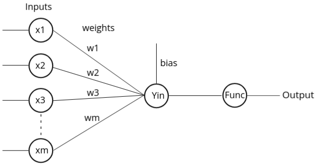
The architecture consists of four main components:
- Inputs: Inputs are the data provided to the neural network. For instance, if there are four inputs, then the network will have four input nodes.
- Weights and Bias: The weights and bias are values between the input and output layers. The weights control the strength of the connection between input and output, and the values typically range between 0 and 1.
- Net Input Function: The net input function is calculated by multiplying the input
values with the respective weights, and
then summing the result. The formula is:
X1 * W1 + X2 * W2 + ... + Xm * Wm + B - Activation Function: After calculating the net input, an activation
function is applied to determine whether
the neuron will "fire" (produce an output). The perceptron typically uses the Step
Activation
Function, which outputs:
- 1 if the net input is greater than a certain threshold value
- 0 if the net input is between a negative and positive threshold
- -1 if the net input is less than the negative threshold
Working of Perceptron
The perceptron operates by comparing the output of the activation function with the target output. If there is a mismatch, the network adjusts the weights and repeats the process until the error is minimized or eliminated.
Perceptron Types
- Single-Layer Perceptron: Consists of only one layer of nodes.
- Multi-Layer Perceptron: Contains two or more layers, allowing for greater processing capability.
Mathematical Formula for Perceptron
The general formula to calculate the output (Y) is:
Y = f(X1 * W1 + X2 * W2 + ... + Xm * Wm + B)
Where f is the activation function. In the step activation function:
\(
f(y) =
\begin{cases}
1 & \text{if } y > \text{threshold} \\
0 & \text{if } -\text{threshold} \leq y \leq +\text{threshold} \\
-1 & \text{if } y < -\text{threshold} \end{cases} \)
Weight Updation
When an error occurs, the weights are updated using the formula:
New Weight = Old Weight + Alpha * T * X
Where:
- Alpha: Learning rate (between 0 and 1)
- T: Target value
- X: Input value
Perceptron Training Algorithm
The training algorithm follows these steps:
- Initialize weights and bias, and set the learning rate (Alpha).
- For each training input pair, calculate the net input:
Y_input = X1 * W1 + X2 * W2 + ... + Xn * Wn + B - Apply the activation function and calculate the output (Y).
- Compare the output (Y) with the target value (T). If they are equal, proceed. If not, update the weights using the formula.
- Repeat this process until there are no further inputs or the error becomes zero.
Flowchart of Perceptron Training
The flowchart of the perceptron training process involves:
- Initializing the weights and bias.
- Calculating the net input and applying the activation function.
- Comparing the output with the target value.
- Updating the weights if necessary.
- Repeating the process until the output matches the target.
Testing Algorithm
After training, the network is tested using the following steps:
- Step 0: Use the weights obtained from the training phase.
- Step 1: For each test input pair, calculate the net input using the same
formula:
Y_input = X1 * W1 + X2 * W2 + ... + Xn * Wn + B - Step 2: Apply the activation function and compare the output with the target value. If they match, the weights are considered correct.
Perceptron Network Implementation for AND Function
Step 1: Initialize Weights and Bias
Weights (W1, W2) = 0
Bias (B) = 0
Step 2: Calculate Net Input (y_input)
y_input = B + Σ(x_i * W_i)
Apply activation function:
\( f(y\_input) =
\begin{cases}
1 & \text{if } y\_input > 0 \\
0 & \text{if } y\_input = 0 \\
-1 & \text{if } y\_input < 0 \end{cases} \)
Step 3: Update Weights and Bias
If y ≠ target, update weights and bias using the formula:
ΔW_i = α * T * x_i (α = 1)
ΔB = α * T
New weights = old weights + ΔW_i
New bias = old bias + ΔB
Truth Table for AND Function
+----+----+--------+
| X1 | X2 | Target |
+----+----+--------+
|  1 |  1 |    1   |
|  1 | -1 |   -1   |
| -1 |  1 |   -1   |
| -1 | -1 |   -1   |
+----+----+--------+
First Approach
+----+----+-------+--------+---------+-----+-----+-----+-----+-----+-----+-----+
| X1 | X2 |   b   | Target | y_input |  y  | ΔW1 | ΔW2 | ΔB  | W1  | W2  |  B  |
|    |    | input |        |         |     |     |     |     | new | new | new |
+----+----+-------+--------+---------+-----+-----+-----+-----+-----+-----+-----+
|  1 |  1 |   1   |   1    |    0    |  0  |  1  |  1  |  1  |  1  |  1  |  1  |
|  1 | -1 |   1   |  -1    |    1    |  1  | -1  |  1  | -1  |  0  |  2  |  0  |
| -1 |  1 |   1   |  -1    |    2    |  1  |  1  | -1  | -1  |  1  |  1  | -1  |
| -1 | -1 |   1   |  -1    |   -3    | -1  |  0  |  0  |  0  |  1  |  1  | -1  |
+----+----+-------+--------+---------+-----+-----+-----+-----+-----+-----+-----+
Final Weights: W1 = 1, W2 = 1, B = -1
Second Approach
+----+----+-------+--------+---------+-----+-----+-----+-----+-----+-----+-----+
| X1 | X2 |   b   | Target | y_input |  y  | ΔW1 | ΔW2 | ΔB  | W1  | W2  |  B  |
|    |    | input |        |         |     |     |     |     | new | new | new |
+----+----+-------+--------+---------+-----+-----+-----+-----+-----+-----+-----+
|  1 |  1 |  -1   |    1   |    1    |  1  |  0  |  0  |  0  |  1  |  1  | -1  |
|  1 | -1 |  -1   |   -1   |   -1    | -1  |  0  |  0  |  0  |  1  |  1  | -1  |
| -1 |  1 |  -1   |   -1   |   -1    | -1  |  0  |  0  |  0  |  1  |  1  | -1  |
| -1 | -1 |  -1   |   -1   |   -3    | -1  |  0  |  0  |  0  |  1  |  1  | -1  |
+----+----+-------+--------+---------+-----+-----+-----+-----+-----+-----+-----+
Final Weights: W1 = 1, W2 = 1, B = -1
Final Weights
W1 = 1
W2 = 1
B = -1
Verification
For input (1, 1), y_input = 1, y = 1 (correct)
For input (1, -1), y_input = -1, y = -1 (correct)
For input (-1, 1), y_input = -1, y = -1 (correct)
For input (-1, -1), y_input = -3, y = -1 (correct)
Delta Learning Rule / Widrow-Hoff Rule
- The Widrow-Hoff rule is a supervised learning algorithm. Supervised learning involves a process where the desired output is compared with the actual output. The difference between the two (error) is used to adjust the weights. This process is repeated iteratively until the actual output is close to the desired output.
- The algorithm uses the difference between the actual output of the neuron and the desired output as the error signal for units in the output layer.
- In Widrow-Hoff learning, the correction to the synaptic weight is proportional to the error signal multiplied by the activation value, which is determined by the derivative of the transfer function.
-
Weight adjustment formula:
Δwnew = α(t - yin) * xi + Δwold
α = learning rate: The learning rate controls how much the weights are adjusted in each iteration. It is a small positive value that ensures gradual convergence.
t = target value: This is the desired output for a given input.
yin = net input to the output unit: This is the weighted sum of inputs to the neuron.
yin: \( \sum_{i=1}^{n} x_i w_i \) - The delta rule is derived from gradient descent, meaning it tries to minimize the error by updating the weights in the direction that reduces the error.
- The perceptron learning rule stops after a finite number of steps, while the gradient descent approach continues indefinitely, converging asymptotically to the solution.