Question:

Let \( X = \{a, b, c, d\} \), \( Y = \{1, 2, 3, 4\} \) and
\( A = \{(a, 0), (b, 0.8), (c, 0.6), (d, 1)\} \)
\( B = \{(1, 0.2), (2, 1), (3, 0.8), (4, 0)\} \)
\( C = \{(1, 0), (2, 0.4), (3, 1), (4, 0.8)\} \)
Here, \( X \) and \( Y \) are sets, and \( A \), \( B \), \( C \) are fuzzy sets.
Determine the implication relations:

• If \( X \) is \( A \), then \( Y \) is \( B \).
• If \( X \) is \( A \), then \( Y \) is \( B \), else \( Y \) is \( C \).

Solution:

If \( X \) is \( A \), then \( Y \) is \( B \):

The implication relation is defined as: \[ R = (A \times B) \cup (A^c \times Y) \]

Step 1: Cartesian Product \( A \times B \)

For \( A \times B \), we calculate the minimum of the membership values of \( A \) and \( B \) for each pair:

\[ A \times B = \begin{pmatrix} \min(0, 0.2) & \min(0, 1) & \min(0, 0.8) & \min(0, 0) \\ \min(0.8, 0.2) & \min(0.8, 1) & \min(0.8, 0.8) & \min(0.8, 0) \\ \min(0.6, 0.2) & \min(0.6, 1) & \min(0.6, 0.8) & \min(0.6, 0) \\ \min(1, 0.2) & \min(1, 1) & \min(1, 0.8) & \min(1, 0) \end{pmatrix} \]

Which simplifies to:

\[ A \times B = \begin{pmatrix} 0 & 0 & 0 & 0 \\ 0.2 & 0.8 & 0.8 & 0 \\ 0.2 & 0.6 & 0.6 & 0 \\ 0.2 & 1 & 0.8 & 0 \end{pmatrix} \]

Step 2: Complement of \( A \), \( A^c \)

The complement \( A^c \) is computed by subtracting each membership value in \( A \) from 1:

\[ A^c = \{(a, 1), (b, 0.2), (c, 0.4), (d, 0)\} \]

Step 3: Cartesian Product \( A^c \times Y \)

For \( A^c \times Y \), we pair each element of \( A^c \) with each element of \( Y \) and compute the minimum of their membership values. Since \( Y = \{(1, 1), (2, 1), (3, 1), (4, 1)\} \), each element in \( Y \) has the membership value of 1:

\[ A^c \times Y = \begin{pmatrix} \min(1, 1) & \min(1, 1) & \min(1, 1) & \min(1, 1) \\ \min(0.2, 1) & \min(0.2, 1) & \min(0.2, 1) & \min(0.2, 1) \\ \min(0.4, 1) & \min(0.4, 1) & \min(0.4, 1) & \min(0.4, 1) \\ \min(0, 1) & \min(0, 1) & \min(0, 1) & \min(0, 1) \end{pmatrix} \]

Which simplifies to:

\[ A^c \times Y = \begin{pmatrix} 1 & 1 & 1 & 1 \\ 0.2 & 0.2 & 0.2 & 0.2 \\ 0.4 & 0.4 & 0.4 & 0.4 \\ 0 & 0 & 0 & 0 \end{pmatrix} \]

Step 4: Union of \( A \times B \) and \( A^c \times Y \)

We now compute the union of \( A \times B \) and \( A^c \times Y \) by taking the element-wise maximum of the two matrices:

\[ R = (A \times B) \cup (A^c \times Y) = \begin{pmatrix} \max(0, 1) & \max(0, 1) & \max(0, 1) & \max(0, 1) \\ \max(0.2, 0.2) & \max(0.8, 0.2) & \max(0.8, 0.2) & \max(0, 0.2) \\ \max(0.2, 0.4) & \max(0.6, 0.4) & \max(0.6, 0.4) & \max(0, 0.4) \\ \max(0.2, 0) & \max(1, 0) & \max(0.8, 0) & \max(0, 0) \end{pmatrix} \]

Which simplifies to:

\[ R = \begin{pmatrix} 1 & 1 & 1 & 1 \\ 0.2 & 0.8 & 0.8 & 0.2 \\ 0.4 & 0.6 & 0.6 & 0.4 \\ 0.2 & 1 & 0.8 & 0 \end{pmatrix} \]

Final Answer:

\[ R = \begin{pmatrix} 1 & 1 & 1 & 1 \\ 0.2 & 0.8 & 0.8 & 0.2 \\ 0.4 & 0.6 & 0.6 & 0.4 \\ 0.2 & 1 & 0.8 & 0 \end{pmatrix} \]

2. If X is A, then Y is B, else Y is C:

For this case, we need to compute \( R = (A \times B) \cup (A^c \times C) \), similar to the previous calculation. However, this step also includes the condition for "else Y is C" when \( X \) is not in \( A \).

Step 1: Complement of A (\(A^c\)) is the same as before:

\[ A^c = \{(a, 1), (b, 0.2), (c, 0.4), (d, 0)\} \]

Step 2: Compute \( A^c \times C \) (same as before):

\[ A^c \times C = \begin{pmatrix} 0 & 0.4 & 1 & 0.8 \\ 0 & 0.2 & 0.2 & 0.2 \\ 0 & 0.4 & 0.4 & 0.4 \\ 0 & 0 & 0 & 0 \end{pmatrix} \]

Step 3: Union of \( (A \times B) \) and \( (A^c \times C) \) (same as before):

R = (A × B) ∪ (A^c × C) = \begin{pmatrix} 0 & 0.4 & 1 & 0.8 \\ 0.2 & 0.8 & 0.8 & 0.2 \\ 0.2 & 0.6 & 0.6 & 0.4 \\ 0.2 & 1 & 0.8 & 0 \end{pmatrix}

This is the final result for the implication relation where "If X is A, then Y is B, else Y is C.

Graphical Representation of Membership Function

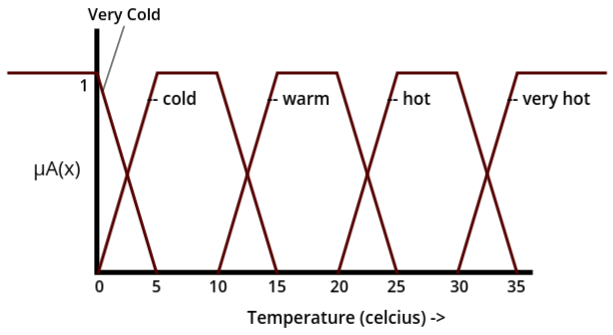
• The membership function represents different temperature categories: [very cold, cold, warm, hot, very hot].
• Let’s understand how the graph works:
  • When the temperature is below 0 degrees Celsius, it fully belongs to the "very cold" category because the membership function (μ_A(x)) value is 1. This means the temperature is completely categorized as "very cold."
  • As the temperature increases from 0 to 5 degrees Celsius, the μ_A(x) value for "very cold" gradually decreases. By the time it reaches 5 degrees Celsius, the μ_A(x) value for "very cold" becomes 0. This indicates that the temperature no longer belongs to the "very cold" category.
  • During the same range (0 to 5 degrees Celsius), the μ_A(x) value for "cold" starts increasing. For example, it might go from 0.1 to 0.2 to 0.3, and so on. At 5 degrees Celsius, the μ_A(x) value for "cold" becomes 1, meaning the temperature fully belongs to the "cold" category.
  • From 5 to 10 degrees Celsius, the temperature remains fully in the "cold" category, as indicated by the μ_A(x) value of 1. A similar pattern is shown for other categories like "warm," "hot," and "very hot" in the graph.

Membership Function Features

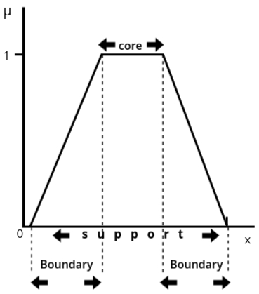
A is a fuzzy set, and x is a member of A. These features of the membership function can be understood by plotting them on a graph:

1. Support: The support of a fuzzy set is the set of all elements x for which the membership value μ_A(x) is greater than 0.
   Meaning: It represents all points where the fuzzy set has some degree of membership, no matter how small.
   Mathematical Representation:
   Support(A) = {x | μ_A(x) > 0}
   Example: If μ_A(x) > 0 for elements x = 1, 2, 3, then the support of the set A is {1, 2, 3}.
2. Core: The core of a fuzzy set is the set of all elements x for which the membership value μ_A(x) is exactly equal to 1.
   Meaning: It represents the points that fully belong to the fuzzy set with the maximum membership value.
   Mathematical Representation:
   Core(A) = {x | μ_A(x) = 1}
   Example: If μ_A(x) = 1 for elements x = 5 and x = 6, then the core of the set A is {5, 6}.
3. Boundary: The boundary of a fuzzy set consists of all elements x where the membership value is strictly between 0 and 1.
   Meaning: It represents the elements that belong to the fuzzy set partially (neither fully included nor completely excluded).
   Mathematical Representation:
   Boundary(A) = {x | 0 < μ_A(x) < 1}
   Example: If μ_A(x) = 0.4 for x = 4 and μ_A(x) = 0.8 for x = 7, then the boundary of the set A includes {4, 7}.

Types of Membership Function

1: Triangular Membership Function

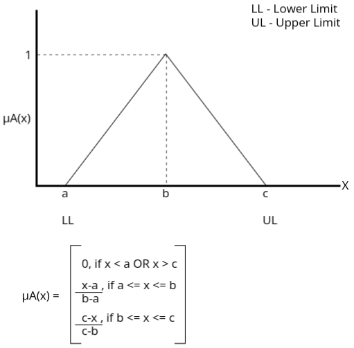
Importance: Simple and computationally efficient, making it ideal for real-time systems. It is widely used due to its linear structure and ease of implementation.

2: Trapezoidal Membership Function

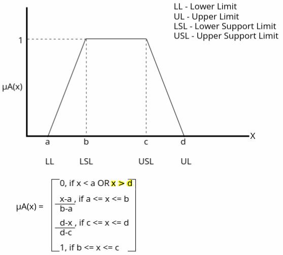
Importance: Extends the triangular membership function by allowing a flat top, providing more flexibility for modeling uncertainties and overlapping ranges in fuzzy systems.

3: Gaussian Membership Function

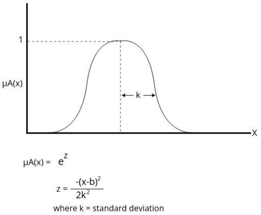
Importance: Smooth and differentiable, making it suitable for applications requiring gradient-based optimization. It is commonly used in control systems and fuzzy inference systems.

4: Sigmoidal Membership Function

This function is mainly used in ANN.

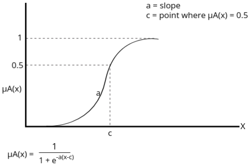
Importance: Offers a smooth transition between membership grades and is particularly useful in artificial neural networks (ANNs) and systems requiring smooth activation functions.

Discrete Membership

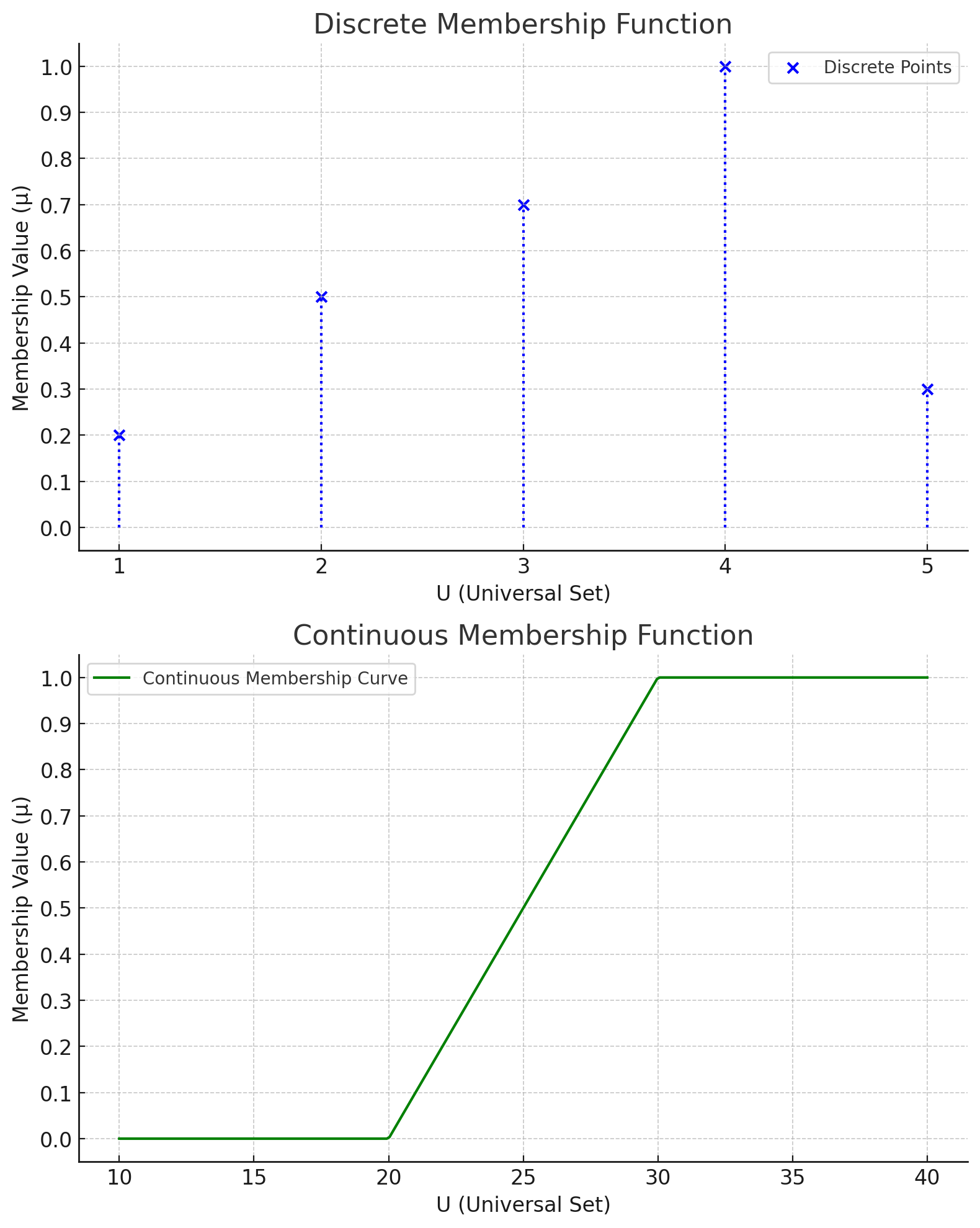
• In a discrete membership function, the membership values are defined only at specific, distinct points in the universal set.
• These points are not continuous and are often represented as a series of individual data points.
• Example: Let U = {1, 2, 3, 4, 5} and the fuzzy set A is defined as:
  A = {(1, 0.2), (2, 0.5), (3, 0.7), (4, 1.0), (5, 0.3)}.
  Here, the membership function μ_A(x) is only defined for these discrete points: 1, 2, 3, 4, and 5.
• Such membership functions are represented graphically as isolated points, often marked with dots or vertical lines.

Continuous Membership

• In a continuous membership function, the membership values are defined over a continuous range of points in the universal set.
• The membership function is expressed as a smooth curve rather than isolated points.
• Example: Let U represent the range of temperatures in degrees Celsius. The fuzzy set "Warm" may be defined by:
  μ_Warm(x) =
  • 0, if x < 20
  • (x - 20) / 10, if 20 ≤ x ≤ 30
  • 1, if x > 30
  
  This membership function defines a smooth transition of values from 0 to 1 as the temperature increases.
• Graphically, a continuous membership function appears as a curve, indicating gradual changes in membership value.

Functional Blocks of FIS

The following five functional blocks are essential for constructing a FIS:

1. Rule Base: It contains a collection of fuzzy if-then rules that define the relationship between input and output variables.
2. Database: It defines the membership functions of fuzzy sets used in the fuzzy rules, providing the necessary information for fuzzification and inference.
3. Decision-Making Unit: This unit applies the fuzzy rules to the input data to derive fuzzy outputs. It combines the results of all applicable rules.
4. Fuzzification Interface Unit: It converts crisp (precise) input values into fuzzy sets using membership functions. This step is crucial for handling imprecise or uncertain data.
5. Defuzzification Interface Unit: It converts the fuzzy output of the inference process into crisp values for actionable results, making the system usable in real-world scenarios.

Understanding Fuzzification and Defuzzification

1. Fuzzification is the process of converting crisp (precise and numerical) input values into fuzzy sets using predefined membership functions. This step allows a system to handle imprecise, uncertain, or vague data by mapping input values to linguistic terms (e.g., "low," "medium," "high") represented as fuzzy sets.
2. Defuzzification is the process of converting fuzzy outputs generated by the inference engine into crisp (precise and numerical) values. It translates the fuzzy results into actionable outputs by applying methods like the centroid of area, bisector, or mean of maxima, making the output usable in real-world scenarios.

Block Diagram of FIS

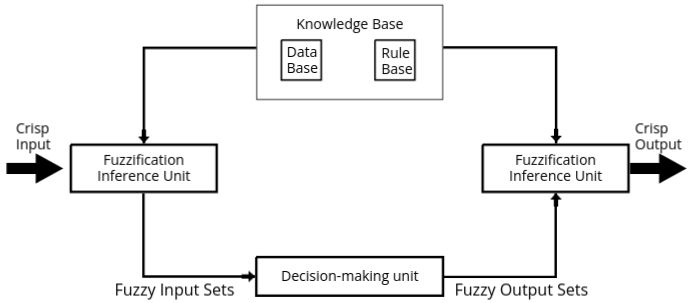
The block diagram of a Fuzzy Inference System (FIS) illustrates the flow of data through its functional components. The diagram typically consists of the following parts:

1. Input: Crisp input values are provided to the system.
2. Fuzzification: Converts crisp inputs into fuzzy sets using membership functions.
3. Inference Engine: Processes fuzzy inputs using the rule base and database to generate fuzzy outputs.
4. Defuzzification: Converts fuzzy outputs into crisp values suitable for real-world use.
5. Output: The final crisp output is delivered, which can be used in decision-making or control applications.

Working of FIS

The working of the Fuzzy Inference System (FIS) consists of the following steps:

1. Fuzzification: The fuzzification unit applies various fuzzification methods to convert crisp input values into fuzzy inputs using membership functions.
2. Knowledge Base: A knowledge base, which includes both the rule base (fuzzy if-then rules) and the database (membership functions), is used to process the fuzzy inputs.
3. Inference Mechanism: The inference engine applies the fuzzy rules to the fuzzy inputs to generate fuzzy outputs. This step combines all applicable rules and determines the degree to which each output is activated.
4. Defuzzification: The defuzzification unit converts the fuzzy output into a crisp output, making it usable for decision-making or control applications in real-world scenarios.

Methods of FIS

The following are the two important methods of Fuzzy Inference Systems, differing in the way they define the consequent of fuzzy rules:

1. Mamdani Fuzzy Inference System: A widely used approach that represents the consequent of fuzzy rules as fuzzy sets. It uses a max-min (or max-product) composition method and requires defuzzification to produce a crisp output.
2. Takagi-Sugeno Fuzzy Model (TS Model): This approach represents the consequent of fuzzy rules as a mathematical function (e.g., linear or constant). It simplifies the defuzzification process and is suitable for control applications requiring precise outputs.

Mamdani Fuzzy Inference System

The Mamdani Fuzzy Inference System is one of the earliest and most popular FIS methods. It is characterized by its use of fuzzy sets for both the antecedent and consequent of rules. The steps involved include:

1. Fuzzification: Converting crisp inputs into fuzzy sets using membership functions.
2. Rule Evaluation: Applying fuzzy rules and combining the results using fuzzy operators (e.g., AND, OR).
3. Aggregation: Combining the outputs of all fuzzy rules into a single fuzzy set.
4. Defuzzification: Converting the aggregated fuzzy set into a crisp output using methods like the centroid or bisector method.

Takagi-Sugeno Fuzzy Model

The Takagi-Sugeno Fuzzy Model is designed for precise and computationally efficient outputs. It differs from the Mamdani method in the following ways:

1. Consequent Representation: The consequent of rules is represented as a linear or constant mathematical function instead of a fuzzy set.
2. Rule Evaluation: The rules are evaluated similarly to Mamdani, but the output is directly calculated using the functions defined in the consequents.
3. Defuzzification: The weighted average method is typically used, making the defuzzification process straightforward and fast.

This model is commonly used in engineering and control systems due to its efficiency and ability to handle large-scale problems.